Data science with R on Google Cloud: Exploratory data analysis

Last reviewed 2024-07-22 UTC

This document shows you how to get started with data science at scale with R on Google Cloud. This is intended for those who have some experience with R and with Jupyter notebooks, and who are comfortable with SQL.

This document focuses on performing exploratory data analysis using Vertex AI Workbench instances and BigQuery. You can find the accompanying code in a Jupyter notebook that's on GitHub.

Overview

R is one of the most widely used programming languages for statistical modeling. It has a large and active community of data scientists and machine learning (ML) professionals. With more than 20,000 packages in the open-source repository of the Comprehensive R Archive Network (CRAN), R has tools for all statistical data analysis applications, ML, and visualization. R has experienced steady growth in the last two decades due to its expressiveness of its syntax, and because of how comprehensive its data and ML libraries are.

As a data scientist, you might want to know how you can make use of your skill set by using R, and how you can also harness the advantages of the scalable, fully managed cloud services for data science.

Architecture

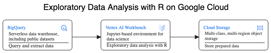
In this walkthrough, you use Vertex AI Workbench instances as the data science environments to perform exploratory data analysis (EDA). You use R on data that you extract in this walkthrough from BigQuery, Google's serverless, highly scalable, and cost-effective cloud data warehouse. After you analyze and process the data, the transformed data is stored in Cloud Storage for further potential ML tasks. This flow is shown in the following diagram:

Example data

The example data for this document is the BigQuery New York City taxi trips dataset. This public dataset includes information about the millions of taxi rides that take place in New York City each year. In this document, you use the data from 2022, which is in the bigquery-public-data.new_york_taxi_trips.tlc_yellow_trips_2022 table in BigQuery.

This document focuses on EDA and on visualization using R and BigQuery. The steps in this document set you up for a ML goal of predicting taxi fare amount (the amount before taxes, fees, and other extras), given a number of factors about the trip. The actual model creation isn't covered in this document.

Vertex AI Workbench

Vertex AI Workbench is a service that offers an integrated JupyterLab environment, with the following features:

• One-click deployment. You can use a single click to start a JupyterLab instance that's preconfigured with the latest machine-learning and data-science frameworks.
• Scale on demand. You can start with a small machine configuration (for example, 4 vCPUs and 16 GB of RAM, as in this document), and when your data gets too big for one machine, you can scale up by adding CPUs, RAM, and GPUs.
• Google Cloud integration. Vertex AI Workbench instances are integrated with Google Cloud services like BigQuery. This integration makes it straightforward to go from data ingestion to preprocessing and exploration.
• Pay-per-use pricing. There are no minimum fees or up-front commitments. For information, see pricing for Vertex AI Workbench. You also pay for the Google Cloud resources that you use within the notebooks (such as BigQuery and Cloud Storage).

Vertex AI Workbench instance notebooks run on Deep Learning VM Images. This document supports creating a Vertex AI Workbench instance that has R 4.3.

Work with BigQuery using R

BigQuery doesn't require infrastructure management, so you can focus on uncovering meaningful insights. You can analyze large amounts of data at scale and prepare datasets for ML by using the rich SQL analytical capabilities of BigQuery.

To query BigQuery data using R, you can use bigrquery, an open-source R library. The bigrquery package provides the following levels of abstraction on top of BigQuery:

• The low-level API provides thin wrappers over the underlying BigQuery REST API.
• The DBI interface wraps the low-level API and makes working with BigQuery similar to working with any other database system. This is the most convenient layer if you want to run SQL queries in BigQuery or upload less than 100 MB.
• The dbplyr interface lets you treat BigQuery tables like in-memory data frames. This is the most convenient layer if you don't want to write SQL, but instead want dbplyr to write it for you.

This document uses the low-level API from bigrquery, without requiring DBI or dbplyr.

Objectives

• Create a Vertex AI Workbench instance that has R support.
• Query and analyze data from BigQuery using the bigrquery R library.
• Prepare and store data for ML in Cloud Storage.

Costs

In this document, you use the following billable components of Google Cloud:

• BigQuery
• Vertex AI Workbench instances. You are also charged for resources used within notebooks, including compute resources, BigQuery, and API requests.
• Cloud Storage

To generate a cost estimate based on your projected usage, use the pricing calculator. New Google Cloud users might be eligible for a free trial.

Before you begin

1. Sign in to your Google Cloud account. If you're new to Google Cloud, create an account to evaluate how our products perform in real-world scenarios. New customers also get $300 in free credits to run, test, and deploy workloads.

2. In the Google Cloud console, on the project selector page, select or create a Google Cloud project.

   Note: If you don't plan to keep the resources that you create in this procedure, create a project instead of selecting an existing project. After you finish these steps, you can delete the project, removing all resources associated with the project.

   Go to project selector

3. Make sure that billing is enabled for your Google Cloud project.

4. Enable the Compute Engine API.

   Enable the API

5. In the Google Cloud console, on the project selector page, select or create a Google Cloud project.

   Note: If you don't plan to keep the resources that you create in this procedure, create a project instead of selecting an existing project. After you finish these steps, you can delete the project, removing all resources associated with the project.

   Go to project selector

6. Make sure that billing is enabled for your Google Cloud project.

7. Enable the Compute Engine API.

   Enable the API

Create a Vertex AI Workbench instance

The first step is to create a Vertex AI Workbench instance that you can use for this walkthrough.

1. In the Google Cloud console, go to the Workbench page.

   Go to Workbench

2. On the Instances tab, click Create New.

3. On the New instance window, click Create. For this walkthrough, keep all of the default values.

   The Vertex AI Workbench instance can take 2-3 minutes to start. When it's ready, the instance is automatically listed in the Notebook instances pane, and an Open JupyterLab link is next to the instance name. If the link to open JupyterLab doesn't appear in the list after a few minutes, then refresh the page.

Open JupyterLab and install R

To complete the walkthrough in the notebook, you need to open the JupyterLab environment, install R, clone the vertex-ai-samples GitHub repository, and then open the notebook.

1. In the instances list, click Open Jupyterlab. This opens the JupyterLab environment in another tab in your browser.

2. In the JupyterLab environment, click  New Launcher, and then on the Launcher tab, click Terminal.

3. In the terminal pane, install R:

   conda create -n r
   conda activate r
   conda install -c r r-essentials r-base=4.3.2
   

   During the installation, each time that you're prompted to continue, type y. The installation might take a few minutes to finish. When the installation is complete, the output is similar to the following:

   done
   Executing transaction: done
   ® jupyter@instance-INSTANCE_NUMBER:~$
   

   Where INSTANCE_NUMBER is the unique number that's assigned to your Vertex AI Workbench instance.

4. After the commands finish executing in the terminal, refresh your browser page, and then open the Launcher by clicking  New Launcher.

   The Launcher tab shows options for launching R in a notebook or in the console, and to create an R file.

5. Click the Terminal tab, and then clone the vertex-ai-samples GitHub repository:

   git clone https://github.com/GoogleCloudPlatform/vertex-ai-samples.git
   

   When the command finishes, you see the vertex-ai-samples folder in the file browser pane of the JupyterLab environment.

6. In the file browser, open vertex-ai-samples>notebooks >community>exploratory_data_analysis. You see the eda_with_r_and_bigquery.ipynb notebook.

Open the notebook and set up R

1. In the file browser, open the eda_with_r_and_bigquery.ipynb notebook.

   This notebook goes through exploratory data analysis with R and BigQuery. Throughout the rest of this document, you work in the notebook, and you run the code that you see within the Jupyter notebook.

2. Check the version of R that the notebook is using:

   version
   

   The version.string field in the output should show R version 4.3.2, which you installed in the previous section.

3. Check for and install the necessary R packages if they aren't already available in the current session:

   # List the necessary packages
   needed_packages <- c("dplyr", "ggplot2", "bigrquery")
   
   # Check if packages are installed
   installed_packages <- .packages(all.available = TRUE)
   missing_packages <- needed_packages[!(needed_packages %in% installed_packages)]
   
   # If any packages are missing, install them
   if (length(missing_packages) > 0) {
     install.packages(missing_packages)
   }
   

4. Load the required packages:

   # Load the required packages
   lapply(needed_packages, library, character.only = TRUE)
   

5. Authenticate bigrquery using out-of-band authentication:

   bq_auth(use_oob = True)
   

6. Set the name of the project that you want to use for this notebook by replacing [YOUR-PROJECT-ID] with a name:

   # Set the project ID
   PROJECT_ID <- "[YOUR-PROJECT-ID]"
   

7. Set the name of the Cloud Storage bucket in which to store output data by replacing [YOUR-BUCKET-NAME] with a globally unique name:

   BUCKET_NAME <- "[YOUR-BUCKET-NAME]"
   

8. Set the default height and width for plots that will be generated later in the notebook:

   options(repr.plot.height = 9, repr.plot.width = 16)
   

Query data from BigQuery

In this section of the notebook, you read the results of executing a BigQuery SQL statement into R and take a preliminary look at the data.

1. Create a BigQuery SQL statement that extracts some possible predictors and the target prediction variable for a sample of trips. The following query filters out some outlier or nonsensical values in the fields that are being read in for analysis.

   sql_query_template <- "
       SELECT
         TIMESTAMP_DIFF(dropoff_datetime, pickup_datetime, MINUTE) AS trip_time_minutes,
   
         passenger_count,
   
         ROUND(trip_distance, 1) AS trip_distance_miles,
   
         rate_code,
         /* Mapping from rate code to type from description column in BigQuery table schema */
         (CASE
           WHEN rate_code = '1.0'
             THEN 'Standard rate'
           WHEN rate_code = '2.0'
             THEN 'JFK'
           WHEN rate_code = '3.0'
             THEN 'Newark'
           WHEN rate_code = '4.0'
             THEN 'Nassau or Westchester'
           WHEN rate_code = '5.0'
             THEN 'Negotiated fare'
           WHEN rate_code = '6.0'
             THEN 'Group ride'
           /* Several NULL AND some '99.0' values go here */
           ELSE 'Unknown'
           END)
           AS rate_type,
   
         fare_amount,
   
         CAST(ABS(FARM_FINGERPRINT(
           CONCAT(
             CAST(trip_distance AS STRING),
             CAST(fare_amount AS STRING)
             )
           ))
           AS STRING)
           AS key
   
       FROM
         `bigquery-public-data.new_york_taxi_trips.tlc_yellow_trips_2022`
   
       /* Filter out some outlier or hard to understand values */
       WHERE
         (TIMESTAMP_DIFF(dropoff_datetime, pickup_datetime, MINUTE)
           BETWEEN 0.01 AND 120)
         AND
         (passenger_count BETWEEN 1 AND 10)
         AND
         (trip_distance BETWEEN 0.01 AND 100)
         AND
         (fare_amount BETWEEN 0.01 AND 250)
   
       LIMIT %s
   "
   

   The key column is a generated row identifier based on the concatenated values of the trip_distance and fare_amount columns.

2. Run the query and retrieve the same data as an in-memory tibble, which is like a data frame.

   sample_size <- 10000
   
   sql_query <- sprintf(sql_query_template, sample_size)
   
   taxi_trip_data <- bq_table_download(
       bq_project_query(
           PROJECT_ID,
           query = sql_query
       )
   )
   

3. View the retrieved results:

   head(taxi_trip_data)
   

   The output is a table that's similar to the following image:

   

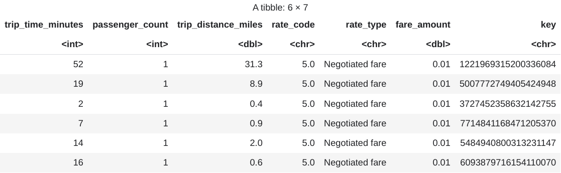
   The results show these columns of trip data:

   • trip_time_minutes integer
   • passenger_count integer
   • trip_distance_miles double
   • rate_code character
   • rate_type character
   • fare_amount double
   • key character

4. View the number of rows and data types of each column:

   str(taxi_trip_data)
   

   The output is similar to the following:

   tibble [10,000 x 7] (S3: tbl_df/tbl/data.frame)
   $ trip_time_minutes  : int [1:10000] 52 19 2 7 14 16 1 2 2 6 ...
   $ passenger_count    : int [1:10000] 1 1 1 1 1 1 1 1 3 1 ...
   $ trip_distance_miles: num [1:10000] 31.3 8.9 0.4 0.9 2 0.6 1.7 0.4 0.5 0.2 ...
   $ rate_code          : chr [1:10000] "5.0" "5.0" "5.0" "5.0" ...
   $ rate_type          : chr [1:10000] "Negotiated fare" "Negotiated fare" "Negotiated fare" "Negotiated fare" ...
   $ fare_amount        : num [1:10000] 0.01 0.01 0.01 0.01 0.01 0.01 0.01 0.01 0.01 0.01 ...
   $ key                : chr [1:10000] "1221969315200336084" 5007772749405424948" "3727452358632142755" "77714841168471205370" ...
   

5. View a summary of the retrieved data:

   summary(taxi_trip_data)
   

   The output is similar to the following:

   trip_time_minutes passenger_count trip_distance_miles  rate_code
   Min.   :  1.00    Min.   :1.000   Min.   : 0.000      Length:10000
   1st Qu.: 20.00    1st Qu.:1.000   1st Qu.: 3.700      Class :character
   Median : 24.00    Median :1.000   Median : 4.800      Mode  :character
   Mean   : 30.32    Mean   :1.465   Mean   : 9.639
   3rd Qu.: 39.00    3rd Qu.:2.000   3rd Qu.:17.600
   Max.   :120.00    Max.   :9.000   Max.   :43.700
   rate_type          fare_amount         key
   Length:10000       Min.   :  0.01   Length:10000
   Class :character   1st Qu.: 16.50   Class :character
   Mode  :character   Median : 16.50   Mode  :character
                     Mean   : 31.22
                     3rd Qu.: 52.00
                     Max.   :182.50
   

Visualize data using ggplot2

In this section of the notebook, you use the ggplot2 library in R to study some of the variables from the example dataset.

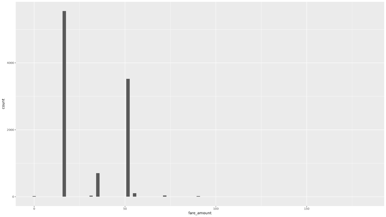
1. Display the distribution of the fare_amount values using a histogram:

   ggplot(
       data = taxi_trip_data,
       aes(x = fare_amount)
       ) +
   geom_histogram(bins = 100)
   

   The resulting plot is similar to the graph in the following image:

   

2. Display the relationship between trip_distance and fare_amount using a scatter plot:

   ggplot(
       data = taxi_trip_data,
       aes(x = trip_distance_miles, y = fare_amount)
       ) +
   geom_point() +
   geom_smooth(method = "lm")
   

   The resulting plot is similar to the graph in the following image:

   

Process the data in BigQuery from R

When you're working with large datasets, we recommend that you perform as much analysis as possible (aggregation, filtering, joining, computing columns, and so on) in BigQuery, and then retrieve the results. Performing these tasks in R is less efficient. Using BigQuery for analysis takes advantage of the scalability and performance of BigQuery, and makes sure that the returned results can fit into memory in R.

1. In the notebook, create a function that finds the number of trips and the average fare amount for each value of the chosen column:

   get_distinct_value_aggregates <- function(column) {
       query <- paste0(
           'SELECT ',
             column,
             ',
             COUNT(1) AS num_trips,
             AVG(fare_amount) AS avg_fare_amount
   
           FROM
             `bigquery-public-data.new_york_taxi_trips.tlc_yellow_trips_2022`
   
           WHERE
             (TIMESTAMP_DIFF(dropoff_datetime, pickup_datetime, MINUTE)
               BETWEEN 0.01 AND 120)
             AND
             (passenger_count BETWEEN 1 AND 10)
             AND
             (trip_distance BETWEEN 0.01 AND 100)
             AND
             (fare_amount BETWEEN 0.01 AND 250)
   
           GROUP BY 1
           '
           )
   
       bq_table_download(
           bq_project_query(
               PROJECT_ID,
               query = query
           )
       )
   }
   

2. Invoke the function using the trip_time_minutes column that is defined using the timestamp functionality in BigQuery:

   df <- get_distinct_value_aggregates(
     'TIMESTAMP_DIFF(dropoff_datetime, pickup_datetime, MINUTE) AS trip_time_minutes')
   
   ggplot(
       data = df,
       aes(x = trip_time_minutes, y = num_trips)
       ) +
   geom_line()
   
   ggplot(
       data = df,
       aes(x = trip_time_minutes, y = avg_fare_amount)
       ) +
   geom_line()
   

   The notebook displays two graphs. The first graph shows the number of trips by length of trip in minutes. The second graph shows the average fare amount of trips by trip time.

   The output of the first ggplot command is as follows, which shows the number of trips by length of trip (in minutes):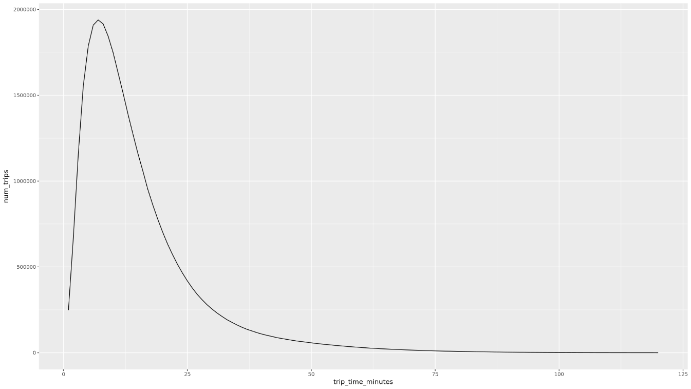

   

   The output of the second ggplot command is as follows, which shows the average fare amount of trips by trip time: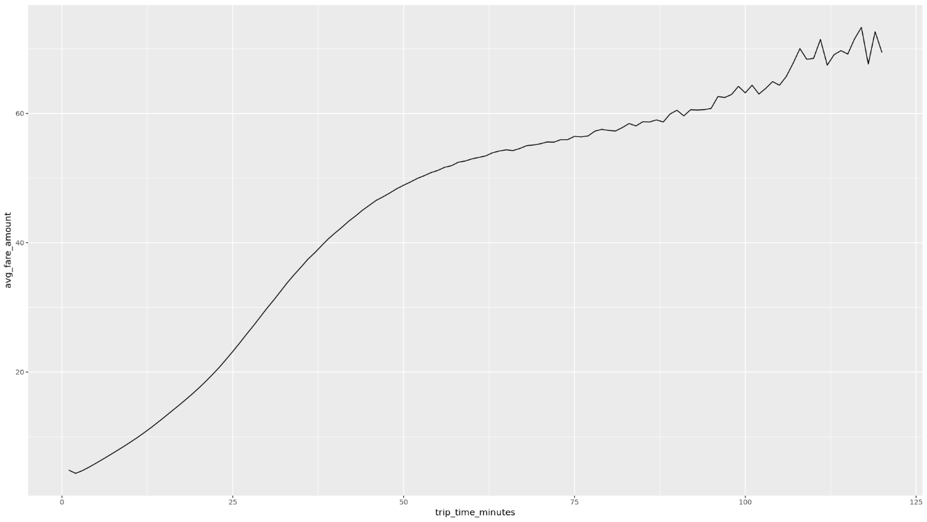

   

   To see more visualization examples with other fields in the data, refer to the notebook.

Save data as CSV files to Cloud Storage

The next task is to save extracted data from BigQuery as CSV files in Cloud Storage so you can use it for further ML tasks.

1. In the notebook, load training and evaluation data from BigQuery into R:

   # Prepare training and evaluation data from BigQuery
   sample_size <- 10000
   
   sql_query <- sprintf(sql_query_template, sample_size)
   
   # Split data into 75% training, 25% evaluation
   train_query <- paste('SELECT * FROM (', sql_query,
     ') WHERE MOD(CAST(key AS INT64), 100) <= 75')
   eval_query <- paste('SELECT * FROM (', sql_query,
     ') WHERE MOD(CAST(key AS INT64), 100) > 75')
   
   # Load training data to data frame
   train_data <- bq_table_download(
       bq_project_query(
           PROJECT_ID,
           query = train_query
       )
   )
   
   # Load evaluation data to data frame
   eval_data <- bq_table_download(
       bq_project_query(
           PROJECT_ID,
           query = eval_query
       )
   )
   

2. Check the number of observations in each dataset:

   print(paste0("Training instances count: ", nrow(train_data)))
   
   print(paste0("Evaluation instances count: ", nrow(eval_data)))
   

   Approximately 75% of the total instances should be in training, with approximately 25% of the remaining instances in evaluation.

3. Write the data to a local CSV file:

   # Write data frames to local CSV files, with headers
   dir.create(file.path('data'), showWarnings = FALSE)
   
   write.table(train_data, "data/train_data.csv",
     row.names = FALSE, col.names = TRUE, sep = ",")
   
   write.table(eval_data, "data/eval_data.csv",
     row.names = FALSE, col.names = TRUE, sep = ",")
   

4. Upload the CSV files to Cloud Storage by wrapping gsutil commands that are passed to the system:

   # Upload CSV data to Cloud Storage by passing gsutil commands to system
   gcs_url <- paste0("gs://", BUCKET_NAME, "/")
   
   command <- paste("gsutil mb", gcs_url)
   
   system(command)
   
   gcs_data_dir <- paste0("gs://", BUCKET_NAME, "/data")
   
   command <- paste("gsutil cp data/*_data.csv", gcs_data_dir)
   
   system(command)
   
   command <- paste("gsutil ls -l", gcs_data_dir)
   
   system(command, intern = TRUE)
   

   You can also upload CSV files to Cloud Storage by using the googleCloudStorageR library, which invokes the Cloud Storage JSON API.

You can also use bigrquery to write data from R back into BigQuery. Writing back to BigQuery is usually done after completing some preprocessing or generating results to be used for further analysis.

Clean up

To avoid incurring charges to your Google Cloud account for the resources used in this document, you should remove them.

Delete the project

The easiest way to eliminate billing is to delete the project you created. If you plan to explore multiple architectures, tutorials, or quickstarts, then reusing projects can help you avoid exceeding project quota limits.

Caution: Deleting a project has the following effects:

• Everything in the project is deleted. If you used an existing project for the tasks in this document, when you delete it, you also delete any other work you've done in the project.
• Custom project IDs are lost. When you created this project, you might have created a custom project ID that you want to use in the future. To preserve the URLs that use the project ID, such as an appspot.com URL, delete selected resources inside the project instead of deleting the whole project.

If you plan to explore multiple architectures, tutorials, or quickstarts, reusing projects can help you avoid exceeding project quota limits.

1. In the Google Cloud console, go to the Manage resources page.

   Go to Manage resources

2. In the project list, select the project that you want to delete, and then click Delete.
3. In the dialog, type the project ID, and then click Shut down to delete the project.

What's next

• Learn more about how you can use BigQuery data in your R notebooks in the bigrquery documentation.
• Learn about best practices for ML engineering in Rules of ML.
• For more reference architectures, diagrams, and best practices, explore the Cloud Architecture Center.

Contributors

Author: Alok Pattani | Developer Advocate

Other contributors:

• Jason Davenport | Developer Advocate
• Firat Tekiner | Senior Product Manager