Measure and tune performance of a TensorFlow inference system

Last reviewed 2023-11-02 UTC

Note: This document or section includes references to one or more terms that Google considers disrespectful or offensive. The terms are used because they are keywords in the software that's described in the document.

This document describes how you measure the performance of the TensorFlow inference system that you created in Deploy a scalable TensorFlow inference system. It also shows you how to apply parameter tuning to improve system throughput.

The deployment is based on the reference architecture described in Scalable TensorFlow inference system.

This series is intended for developers who are familiar with Google Kubernetes Engine and machine learning (ML) frameworks, including TensorFlow and TensorRT.

This document isn't intended to provide the performance data of a particular system. Instead, it offers general guidance on the performance measurement process. The performance metrics that you see, such as for Total Requests per Second (RPS) and Response Times (ms), will vary depending on the trained model, software versions, and hardware configurations that you use.

Architecture

For an architecture overview of the TensorFlow inference system, see Scalable TensorFlow inference system.

Objectives

• Define the performance objective and metrics
• Measure baseline performance
• Perform graph optimization
• Measure FP16 conversion
• Measure INT8 quantization
• Adjust the number of instances

Costs

For details about the costs associated with the deployment, see Costs.

When you finish the tasks that are described in this document, you can avoid continued billing by deleting the resources that you created. For more information, see Clean up.

Before you begin

Ensure that you have already completed the steps in Deploy a scalable TensorFlow inference system.

In this document, you use the following tools:

• An SSH terminal of the working instance that you prepared in Create a working environment.
• The Grafana dashboard that you prepared in Deploy monitoring servers with Prometheus and Grafana.
• The Locust console that you prepared in Deploy a load testing tool.

Set the directory

1. In the Google Cloud console, go to Compute Engine > VM instances.

   Go to VM Instances

   You see the working-vm instance that you created.

2. To open the terminal console of the instance, click SSH.

3. In the SSH terminal, set the current directory to the client subdirectory:

   cd $HOME/gke-tensorflow-inference-system-tutorial/client
   

   In this document, you run all commands from this directory.

Define the performance objective

When you measure performance of inference systems, you must define the performance objective and appropriate performance metrics according to the use case of the system. For demonstration purposes, this document uses the following performance objectives:

• At least 95% of requests receive responses within 100 ms.
• Total throughput, which is represented by requests per second (RPS), improves without breaking the previous objective.

Using these assumptions, you measure and improve the throughput of the following ResNet-50 models with different optimizations. When a client sends inference requests, it specifies the model using the model name in this table.

Model name	Optimization
original	Original model (no optimization with TF-TRT)
tftrt_fp32	Graph optimization (batch size: 64, instance groups: 1)
tftrt_fp16	Conversion to FP16 in addition to the graph optimization (batch size: 64, instance groups: 1)
tftrt_int8	Quantization with INT8 in addition to the graph optimization (batch size: 64, instance groups: 1)
tftrt_int8_bs16_count4	Quantization with INT8 in addition to the graph optimization (batch size: 16, instance groups: 4)

Measure baseline performance

You start by using TF-TRT as a baseline to measure the performance of the original, non-optimized model. You compare the performance of other models with the original to quantitatively evaluate the performance improvement. When you deployed Locust, it was already configured to send requests for the original model.

1. Open the Locust console that you prepared in Deploy a load testing tool.

2. Confirm that the number of clients (referred to as slaves) is 10.

   If the number is less than 10, the clients are still starting up. In that case, wait a few minutes until it becomes 10.

3. Measure the performance:

   1. In the Number of users to simulate field, enter 3000.
   2. In the Hatch rate field, enter 5.
   3. To increase the number of simulated uses by 5 per second until it reaches 3000, click Start swarming.

4. Click Charts.

   The graphs show the performance results. Note that while the Total Requests per Second value linearly increases, the Response Times (ms) value increases accordingly.

   

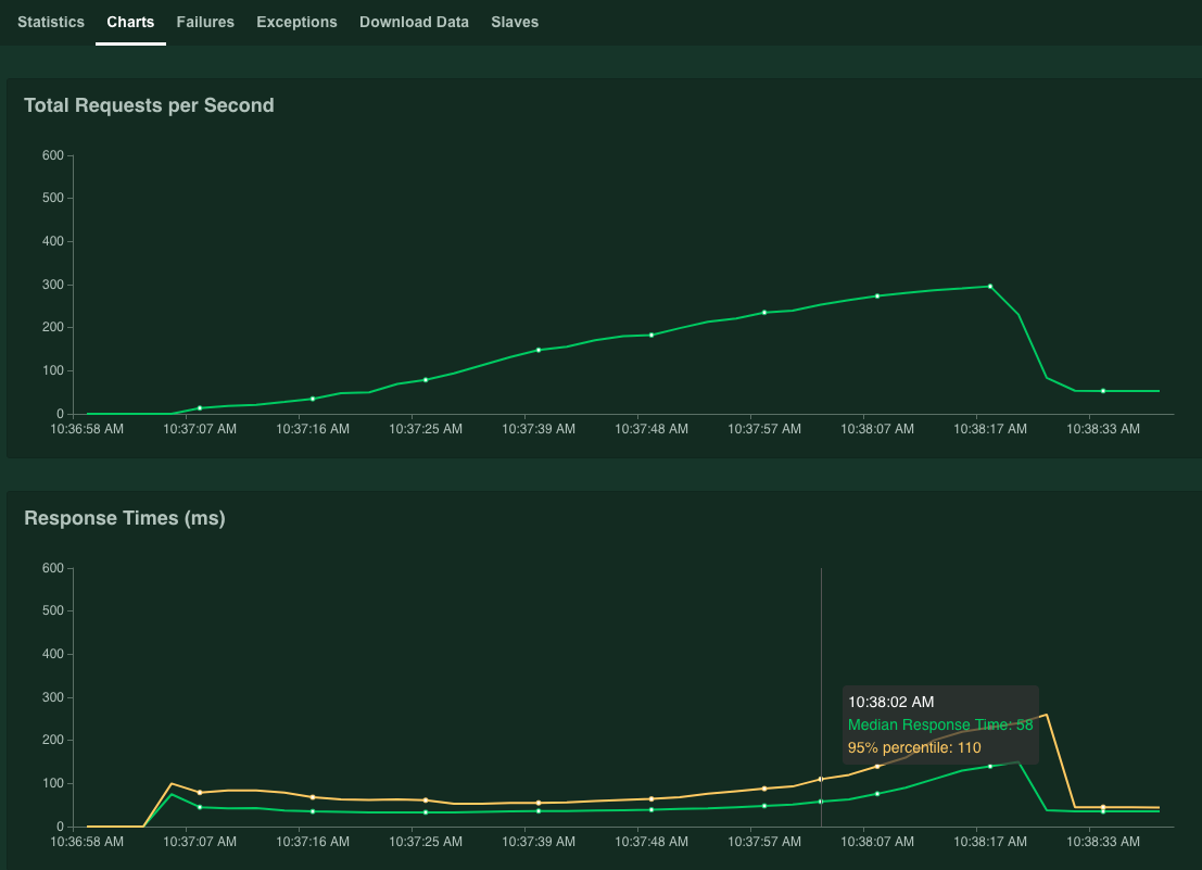
5. When the 95% percentile of Response Times value exceeds 100 ms, click Stop to stop the simulation.

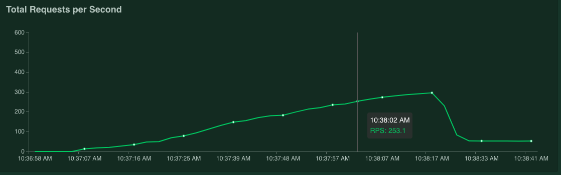
   If you hold the pointer over the graph, you can check the number of requests per second corresponding to when the value of 95% percentile of Response Times exceeded 100 ms.

   For example, in the following screenshot, the number of requests per second is 253.1.

   

   We recommend that you repeat this measurement several times and take an average to account for fluctuation.

6. In the SSH terminal, restart Locust:

   kubectl delete -f deployment_master.yaml -n locust
   kubectl delete -f deployment_slave.yaml -n locust
   kubectl apply -f deployment_master.yaml -n locust
   kubectl apply -f deployment_slave.yaml -n locust
   

7. To repeat the measurement, repeat this procedure.

   Note: Particularly for the first measurement, the response time might be larger because the inference server needs to load the model into memory. In that case, use data from after the second measurement.

Optimize graphs

In this section, you measure the performance of the model tftrt_fp32, which is optimized with TF-TRT for graph optimization. This is a common optimization that is compatible with most of the NVIDIA GPU cards.

1. In the SSH terminal, restart the load testing tool:

   kubectl delete configmap locust-config -n locust
   kubectl create configmap locust-config \
       --from-literal model=tftrt_fp32 \
       --from-literal saddr=${TRITON_IP} \
       --from-literal rps=10 -n locust
   kubectl delete -f deployment_master.yaml -n locust
   kubectl delete -f deployment_slave.yaml -n locust
   kubectl apply -f deployment_master.yaml -n locust
   kubectl apply -f deployment_slave.yaml -n locust
   

   The configmap resource specifies the model as tftrt_fp32.

2. Restart the Triton server:

   kubectl scale deployment/inference-server --replicas=0
   kubectl scale deployment/inference-server --replicas=1
   

   Wait a few minutes until the server processes become ready.

3. Check the server status:

   kubectl get pods
   

   The output is similar to the following, in which the READY column shows the server status:

   NAME                                READY   STATUS    RESTARTS   AGE
   inference-server-74b85c8c84-r5xhm   1/1     Running   0          46s
   

   The value 1/1 in the READY column indicates that the server is ready.

4. Measure the performance:

   1. In the Number of users to simulate field, enter 3000.
   2. In the Hatch rate field, enter 5.
   3. To increase the number of simulated uses by 5 per second until it reaches 3000, click Start swarming.

   The graphs show the performance improvement of the TF-TRT graph optimization.

   For example, your graph might show that the number of requests per second is now 381 with a median response time of 59 ms.

Convert to FP16

In this section, you measure the performance of the model tftrt_fp16, which is optimized with TF-TRT for graph optimization and FP16 conversion. This is an optimization available for NVIDIA T4.

1. In the SSH terminal, restart the load testing tool:

   kubectl delete configmap locust-config -n locust
   kubectl create configmap locust-config \
       --from-literal model=tftrt_fp16 \
       --from-literal saddr=${TRITON_IP} \
       --from-literal rps=10 -n locust
   kubectl delete -f deployment_master.yaml -n locust
   kubectl delete -f deployment_slave.yaml -n locust
   kubectl apply -f deployment_master.yaml -n locust
   kubectl apply -f deployment_slave.yaml -n locust
   

2. Restart the Triton server:

   kubectl scale deployment/inference-server --replicas=0
   kubectl scale deployment/inference-server --replicas=1
   

   Wait a few minutes until the server processes become ready.

3. Measure the performance:

   1. In the Number of users to simulate field, enter 3000.
   2. In the Hatch rate field, enter 5.
   3. To increase the number of simulated uses by 5 per second until it reaches 3000, click Start swarming.

   The graphs show the performance improvement of the FP16 conversion in addition to the TF-TRT graph optimization.

   For example, your graph might show that the number of requests per second is 1072.5 with a median response time of 63 ms.

Quantize with INT8

In this section, you measure the performance of the model tftrt_int8, which is optimized with TF-TRT for graph optimization and INT8 quantization. This optimization is available for NVIDIA T4.

1. In the SSH terminal, restart the load testing tool.

   kubectl delete configmap locust-config -n locust
   kubectl create configmap locust-config \
       --from-literal model=tftrt_int8 \
       --from-literal saddr=${TRITON_IP} \
       --from-literal rps=10 -n locust
   kubectl delete -f deployment_master.yaml -n locust
   kubectl delete -f deployment_slave.yaml -n locust
   kubectl apply -f deployment_master.yaml -n locust
   kubectl apply -f deployment_slave.yaml -n locust
   

2. Restart the Triton server:

   kubectl scale deployment/inference-server --replicas=0
   kubectl scale deployment/inference-server --replicas=1
   

   Wait a few minutes until the server processes become ready.

3. Measure the performance:

   1. In the Number of users to simulate field, enter 3000.
   2. In the Hatch rate field, enter 5.
   3. To increase the number of simulated uses by 5 per second until it reaches 3000, click Start swarming.

   The graphs show the performance results.

   For example, your graph might show that the number of requests per second is 1085.4 with a median response time of 32 ms.

   In this example, the result isn't a significant increase in performance when compared to the FP16 conversion. In theory, the NVIDIA T4 GPU can handle INT8 quantization models faster than FP16 conversion models. In this case, there might be a bottleneck other than GPU performance. You can confirm it from the GPU utilization data on the Grafana dashboard. For example, if utilization is less than 40%, that means that the model cannot fully use the GPU performance.

   As the next section shows, you might be able to ease this bottleneck by increasing the number of instance groups. For example, increase the number of instance groups from 1 to 4, and decrease the batch size from 64 to 16. This approach keeps the total number of requests processed on a single GPU at 64.

Adjust the number of instances

In this section, you measure the performance of the model tftrt_int8_bs16_count4. This model has the same structure as tftrt_int8, but you change the batch size and number of instance groups as described in Quantize with INT8.

1. In the SSH terminal, restart Locust:

   kubectl delete configmap locust-config -n locust
   kubectl create configmap locust-config \
       --from-literal model=tftrt_int8_bs16_count4 \
       --from-literal saddr=${TRITON_IP} \
       --from-literal rps=10 -n locust
   kubectl delete -f deployment_master.yaml -n locust
   kubectl delete -f deployment_slave.yaml -n locust
   kubectl apply -f deployment_master.yaml -n locust
   kubectl apply -f deployment_slave.yaml -n locust
   kubectl scale deployment/locust-slave --replicas=20 -n locust
   

   In this command, you use the configmap resource to specify the model as tftrt_int8_bs16_count4. You also increase the number of Locust client Pods to generate enough workloads to measure the performance limitation of the model.

2. Restart the Triton server:

   kubectl scale deployment/inference-server --replicas=0
   kubectl scale deployment/inference-server --replicas=1
   

   Wait a few minutes until the server processes become ready.

3. Measure the performance:

   1. In the Number of users to simulate field, enter 3000.
   2. In the Hatch rate field, enter 15. For this model, it might take a long time to reach the performance limit if the Hatch rate is set to 5.
   3. To increase the number of simulated uses by 5 per second until it reaches 3000, click Start swarming.

   The graphs show the performance results.

   For example, your graph might show that the number of requests per second is 2236.6 with a median response time of 38 ms.

   By adjusting the number of instances, you can almost double requests per second. Notice that the GPU utilization has increased on the Grafana dashboard (for example, utilization might reach 75%).

Performance and multiple nodes

When scaling with multiple nodes, you measure the performance of a single Pod. Because the inference processes are executed independently on different Pods in a shared-nothing manner, you can assume that the total throughput would scale linearly with the number of Pods. This assumption applies as long as there are no bottlenecks such as network bandwidth between clients and inference servers.

However, it's important to understand how inference requests are balanced among multiple inference servers. Triton uses the gRPC protocol to establish a TCP connection between a client and a server. Because Triton reuses the established connection for sending multiple inference requests, requests from a single client are always sent to the same server. To distribute requests for multiple servers, you must use multiple clients.

Note: The gRPC client module used in Locust has a problem distributing requests for multiple servers. Don't use Locust to measure Triton performance by using a multiple-node configuration.

Clean up

To avoid incurring charges to your Google Cloud account for the resources used in this series, you can delete the project.

Delete the project

Caution: Deleting a project has the following effects:
• Everything in the project is deleted. If you used an existing project for the tasks in this document, when you delete it, you also delete any other work you've done in the project.
• Custom project IDs are lost. When you created this project, you might have created a custom project ID that you want to use in the future. To preserve the URLs that use the project ID, such as an appspot.com URL, delete selected resources inside the project instead of deleting the whole project.
1. In the Google Cloud console, go to the Manage resources page.

   Go to Manage resources

2. In the project list, select the project that you want to delete, and then click Delete.
3. In the dialog, type the project ID, and then click Shut down to delete the project.

What's next

• Learn about configuring compute resources for prediction.
• Learn more about Google Kubernetes Engine (GKE).
• Learn more about Cloud Load Balancing.
• For more reference architectures, diagrams, and best practices, explore the Cloud Architecture Center.