Oracle to BigQuery migration
This document provides high-level guidance on how to migrate from Oracle to BigQuery. It describes the fundamental architectural differences and suggesting ways of migration from data warehouses and data marts running on Oracle RDBMS (including Exadata) to BigQuery. This document provides details that can apply to Exadata, ExaCC, and Oracle Autonomous Data Warehouse also, as they use compatible Oracle software.
This document is for enterprise architects, DBAs, application developers, and IT security professionals who want to migrate from Oracle to BigQuery and solve technical challenges in the migration process.
You can also use batch SQL translation to migrate your SQL scripts in bulk, or interactive SQL translation to translate ad hoc queries. Oracle SQL, PL/SQL, and Exadata are supported by both tools in preview.
Pre-migration
To ensure a successful data warehouse migration, start planning your migration strategy early in your project timeline. For information about how to systematically plan your migration work, see What and how to migrate: The migration framework.
BigQuery capacity planning
Under the hood, analytics throughput in BigQuery is measured in slots. A BigQuery slot is Google's proprietary unit of computational capacity required to execute SQL queries.
BigQuery continuously calculates how many slots are required by queries as they execute, but it allocates slots to queries based on a fair scheduler.
You can choose between the following pricing models when capacity planning for BigQuery slots:
On-demand pricing: Under on-demand pricing, BigQuery charges for the number of bytes processed (data size), so you pay only for the queries that you run. For more information about how BigQuery determines data size, see Data size calculation. Because slots determine the underlying computational capacity, you can pay for BigQuery usage depending on the number of slots you need (instead of bytes processed). By default, Google Cloud projects are limited to a maximum of 2,000 slots.
Capacity-based pricing: With capacity-based pricing, you purchase BigQuery slot reservations (a minimum of 100) instead of paying for the bytes processed by queries that you run. We recommend capacity-based pricing for enterprise data warehouse workloads, which commonly see many concurrent reporting and extract-load-transform (ELT) queries that have predictable consumption.
To help with slot estimation, we recommend setting up BigQuery monitoring using Cloud Monitoring and analyzing your audit logs using BigQuery. Many customers use Looker Studio (for example, see an open source example of a Looker Studio dashboard), Looker, or Tableau as frontends to visualize BigQuery audit log data, specifically for slot usage across queries and projects. You can also leverage BigQuery system tables data for monitoring slot utilization across jobs and reservations. For an example, see an open source example of a Looker Studio dashboard.
Regularly monitoring and analyzing your slot utilization helps you estimate how many total slots your organization needs as you grow on Google Cloud.
For example, suppose you initially reserve 4,000 BigQuery slots to run 100 medium-complexity queries simultaneously. If you notice high wait times in the execution plans of your queries, and your dashboards show high slot utilization, this could indicate that you need additional BigQuery slots to help support your workloads. If you want to purchase slots yourself through yearly or three-year commitments, you can get started with BigQuery reservations using the Google Cloud console or the bq command-line tool.
For any questions related to your current plan and the preceding options, contact your sales representative.
Security in Google Cloud
The following sections describe common Oracle security controls and how you can ensure that your data warehouse stays protected in a Google Cloud environment.
Identity and Access Management (IAM)
Oracle provides users, privileges, roles, and profiles to manage access to resources.
BigQuery uses IAM to manage access to resources and provides centralized access management to resources and actions. The types of resources available in BigQuery include organizations, projects, datasets, tables, and views. In the IAM policy hierarchy, datasets are child resources of projects. A table inherits permissions from the dataset that contains it.
To grant access to a resource, assign one or more roles to a user, group, or service account. Organization and project roles affect the ability to run jobs or manage the project, whereas dataset roles affect the ability to access or modify the data inside a project.
IAM provides these types of roles:
- Predefined roles are meant to support common use cases and access control patterns. Predefined roles provide granular access for a specific service and are managed by Google Cloud.
Basic roles include the Owner, Editor, and Viewer roles.
Custom roles provide granular access according to a user-specified list of permissions.
When you assign both predefined and basic roles to a user, the permissions granted are a union of the permissions of each individual role.
Row-level security
Oracle Label Security (OLS) allows the restriction of data access on a row-by-row basis. A typical use case for row-level security is restricting a sales person's access to the accounts they manage. By implementing row-level security, you gain fine-grained access control.
To achieve row-level security in BigQuery, you can use authorized views and row-level access policies. For more information about how to design and implement these policies, see Introduction to BigQuery row-level security.
Full-disk encryption
Oracle offers Transparent Data Encryption (TDE) and network encryption for data-at-rest and in-transit encryption. TDE requires the Advanced Security option, which is licensed separately.
BigQuery encrypts all data at rest and in transit by default regardless of the source or any other condition, and this cannot be turned off. BigQuery also supports customer-managed encryption keys (CMEK) for users who want to control and manage key encryption keys in Cloud Key Management Service. For more information about encryption at Google Cloud, see Default encryption at rest and Encryption in transit.
Data masking and redaction
Oracle uses data masking in Real Application Testing and data redaction, which lets you mask (redact) data that is returned from queries issued by applications.
BigQuery supports dynamic data masking at the column level. You can use data masking to selectively obscure column data for groups of users, while still allowing access to the column.
You can use the Sensitive Data Protection to identify and redact sensitive personally identifiable information (PII) on BigQuery.
BigQuery and Oracle comparison
This section describes the key differences between BigQuery and Oracle. These highlights help you identify migration hurdles and plan for the changes required.
System architecture
One of the main differences between Oracle and BigQuery is that BigQuery is a serverless cloud EDW with separate storage and compute layers that can scale based on the needs of the query. Given the nature of the BigQuery serverless offering, you are not limited by hardware decisions; instead you can request more resources for your queries and users through reservations. BigQuery also does not require configuration of the underlying software and infrastructure such as operating system (OS), network systems, and storage systems including scaling and high-availability. BigQuery takes care of scalability, management, and administrative operations. The following diagram illustrates the BigQuery storage hierarchy.
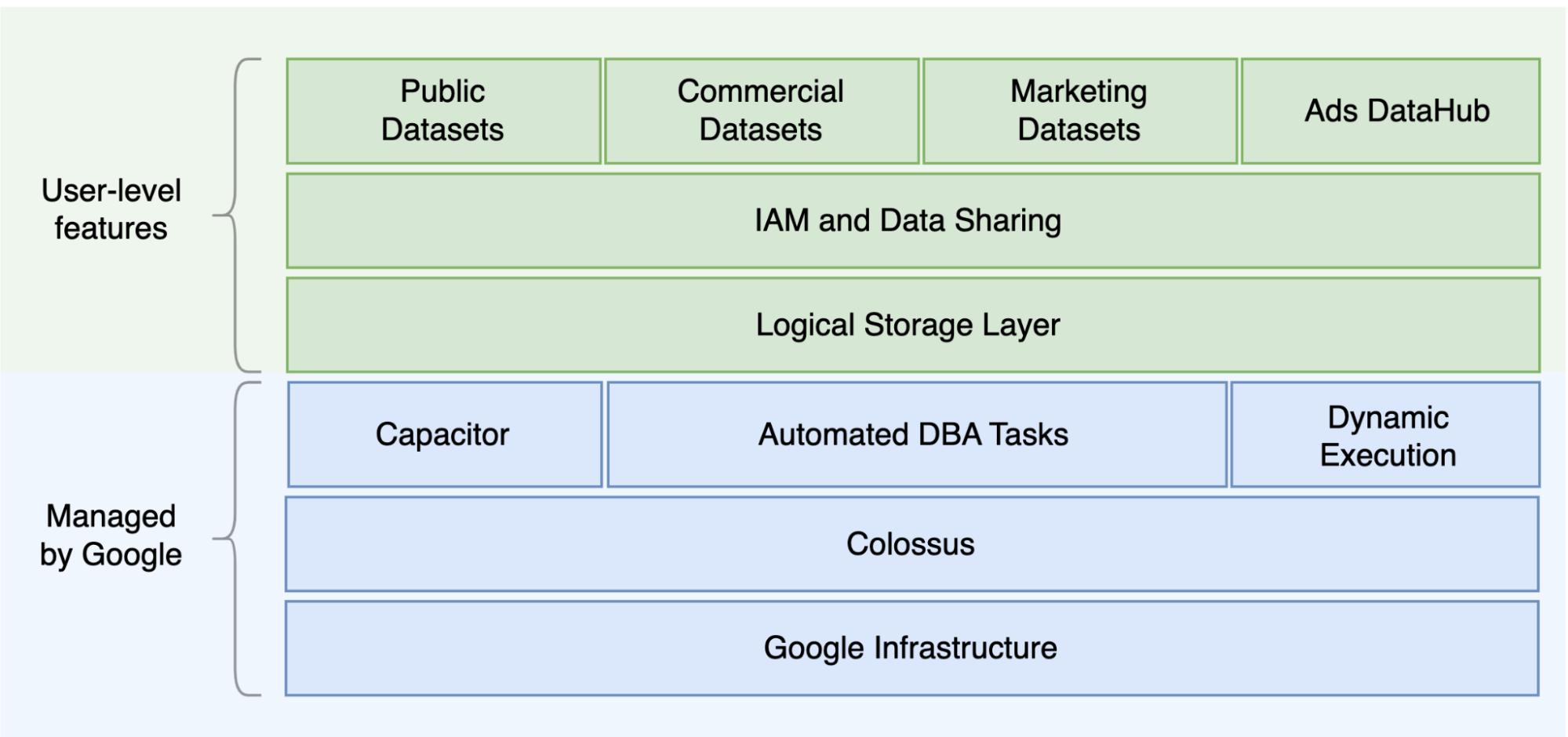
Knowledge of the underlying storage and query processing architecture such as separation between storage (Colossus) and query execution (Dremel) and how Google Cloud allocates resources (Borg) can be good for understanding behavioral differences and optimizing query performance and cost effectiveness. For details, see the reference system architectures for BigQuery, Oracle, and Exadata.
Data and storage architecture
The data and storage structure is an important part of any data analytics system because it affects query performance, cost, scalability, and efficiency.
BigQuery decouples data storage and compute and stores data in Colossus, in which data is compressed and stored in a columnar format called Capacitor.
BigQuery operates directly on compressed data without decompressing by using Capacitor. BigQuery provides datasets as the highest-level abstraction to organize access to tables as shown in the preceding diagram. Schemas and labels can be used for further organization of tables. BigQuery offers partitioning to improve query performance and costs and to manage information lifecycle. Storage resources are allocated as you consume them and deallocated as you remove data or drop tables.
Oracle stores data in row format using Oracle block format organized in segments. Schemas (owned by users) are used to organize tables and other database objects. As of Oracle 12c, multitenant is used to create pluggable databases within one database instance for further isolation. Partitioning can be used to improve query performance and information lifecycle operations. Oracle offers several storage options for standalone and Real Application Clusters (RAC) databases such as ASM, an OS file system, and a cluster file system.
Exadata provides optimized storage infrastructure in storage cell servers and allows Oracle servers to access this data transparently by utilizing ASM. Exadata offers Hybrid Columnar Compression (HCC) options so that users can compress tables and partitions.
Oracle requires pre-provisioned storage capacity, careful sizing, and autoincrement configurations on segments, datafiles, and tablespaces.
Query execution and performance
BigQuery manages performance and scales on the query level to maximize performance for the cost. BigQuery uses many optimizations, for example:
- In-memory query execution
- Multilevel tree architecture based on Dremel execution engine
- Automatic storage optimization within Capacitor
- 1 petabit per second total bisection bandwidth with Jupiter
- Autoscaling resource management to provide fast petabyte-scale queries
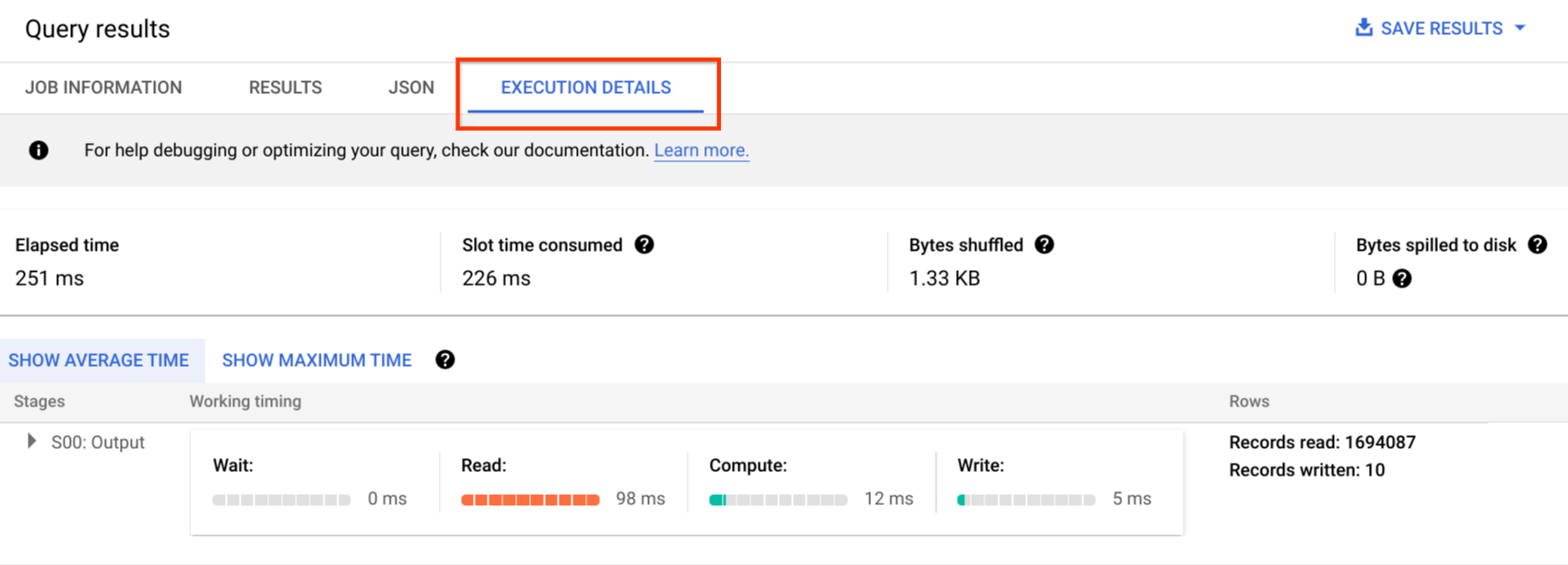
BigQuery gathers column statistics while loading the data and includes diagnostic query plan and timing information. Query resources are allocated according to query type and complexity. Each query uses some number of slots, which are units of computation that includes certain amount of CPU and RAM.
Oracle provides data statistics gathering jobs. The database optimizer uses statistics to provide optimal execution plans. Indexes might be needed for fast row lookups and join operations. Oracle also provides an in-memory column store for in-memory analytics. Exadata provides several performance improvements such as cell smart scan, storage indexes, flash cache, and InfiniBand connections between storage servers and database servers. Real Application Clusters (RAC) can be used for achieving server high availability and scaling database CPU-intensive applications using the same underlying storage.
Optimizing query performance with Oracle requires careful consideration of these options and database parameters. Oracle provides several tools such as Active Session History (ASH), Automatic Database Diagnostic Monitor (ADDM), Automatic Workload Repository (AWR) reports, SQL monitoring and Tuning Advisor, and Undo and Memory Tuning Advisors for performance tuning.
Agile analytics
In BigQuery you can enable different projects, users, and groups to query datasets in different projects. Separation of query execution lets autonomous teams work within their projects without affecting other users and projects by separating slot quotas and querying billing from other projects and the projects that host the datasets.
High availability, backups, and disaster recovery
Oracle provides Data Guard as a disaster recovery and database replication solution. Real Application Clusters (RAC) can be configured for server availability. Recovery Manager (RMAN) backups can be configured for database and archivelog backups and also used for restore and recovery operations. The Flashback database feature can be used for database flashbacks to rewind the database to a specific point in time. Undo tablespace holds table snapshots. It is possible to query old snapshots with the flashback query and "as of" query clauses depending on the DML/DDL operations done previously and the undo retention settings. In Oracle, the whole integrity of the database should be managed within tablespaces that depend on the system metadata, undo, and corresponding tablespaces, because strong consistency is important for Oracle backup, and recovery procedures should include full primary data. You can schedule exports on the table schema level if point-in-time recovery is not needed in Oracle.
BigQuery is fully managed and different from traditional database systems in its complete backup functionality. You don't need to consider server, storage failures, system bugs, and physical data corruptions. BigQuery replicates data across different data centers depending on the dataset location to maximize reliability and availability. BigQuery multi-region functionality replicates data across different regions and protects against unavailability of a single zone within the region. BigQuery single-region functionality replicates data across different zones within the same region.
BigQuery lets you query historical snapshots of tables up to
seven days and restore deleted tables within two days by using time travel.
You can copy a deleted table (in order
to restore it) by using the snapshot
syntax (dataset.table@timestamp).
You can export data from
BigQuery tables for additional backup needs such as to recover
from accidental user operations. Proven backup strategy and schedules used for
existing data warehouse (DWH) systems can be used for backups.
Batch operations and the snapshotting technique allow different backup strategies for BigQuery, so you don't need to export unchanged tables and partitions frequently. One export backup of the partition or table is enough after the load or ETL operation finishes. To reduce backup cost, you can store export files in Cloud Storage Nearline Storage or Coldline Storage and define a lifecycle policy to delete files after a certain amount of time, depending on the data retention requirements.
Caching
BigQuery offers per-user cache, and if data doesn't change, results of queries are cached for approximately 24 hours. If the results are retrieved from the cache, the query costs nothing.
Oracle offers several caches for data and query results such as buffer cache, result cache, Exadata Flash Cache, and in-memory column store.
Connections
BigQuery handles connection management and does not require you
to do any server-side configuration. BigQuery provides JDBC and
ODBC drivers. You can use the
Google Cloud console or the
bq command-line tool for interactive
querying. You can use REST APIs and client
libraries to
programmatically interact with BigQuery You can connect
Google Sheets
directly with BigQuery and use ODBC and JDBC drivers
to connect to Excel. If you are looking for a desktop client, there are free
tools like DBeaver.
Oracle provides listeners, services, service handlers, several configuration and tuning parameters, and shared and dedicated servers to handle database connections. Oracle provides JDBC, JDBC Thin, ODBCdrivers, Oracle Client, and TNSconnections. Scan listeners, scan IP addresses, and scan-name are needed for RAC configurations.
Pricing and licensing
Oracle requires license and support fees based on the core counts for Database editions and Database options such as RAC, multitenant, Active Data Guard, partitioning, in-memory, Real Application Testing, GoldenGate, and Spatial and Graph.
BigQuery offers flexible pricing options based on storage, query, and streaming inserts usage. BigQuery offers capacity-based pricing for customers who need predictable cost and slot capacity in specific regions. Slots that are used for streaming inserts and loads are not counted on project slot capacity. To decide how many slots you want to purchase for your data warehouse, see BigQuery capacity planning.
BigQuery also automatically cuts storage costs in half for unmodified data stored for more than 90 days.
Labeling
BigQuery datasets, tables, and views can be labeled with key-value pairs. Labels can be used for differentiating storage costs and internal chargebacks.
Monitoring and audit logging
Oracle provides different levels and kinds of database auditing options and audit vault and database firewall features, which are licensed separately. Oracle provides Enterprise Manager for database monitoring.
For BigQuery, Cloud Audit Logs is used for both data access logs and audit logs, which are enabled by default. The data access logs are available for 30 days, and the other system events and admin activity logs are available for 400 days. If you need longer retention, you can export logs to BigQuery, Cloud Storage, or Pub/Sub as described in Security log analytics in Google Cloud. If integration with an existing incident monitoring tool is needed, Pub/Sub can be used for exports, and custom development should be done on the existing tool to read logs from Pub/Sub.
Audit logs include all the API calls, query statements, and job statuses. You can use Cloud Monitoring to monitor slot allocation, bytes scanned in queries and stored, and other BigQuery metrics. BigQuery query plan and timeline can be used to analyze query stages and performance.
You can use the error messages table for troubleshooting query job and API errors. To distinguish slot allocations per query or job, you can use this utility, which is beneficial for customers that use capacity-based pricing and have many projects distributed across several teams.
Maintenance, upgrades, and versions
BigQuery is a fully managed service and does not require you to do any maintenance or upgrades. BigQuery does not offer different versions. Upgrades are continuous and don't require downtime or hinder system performance. For more information, see Release notes.
Oracle and Exadata require you to do database and underlying infrastructure-level patching, upgrades, and maintenance. There are many versions of Oracle and a new major version is planned to be released every year. Although new versions are backward-compatible, query performance, context, and features can change.
There can be applications that require specific versions such as 10g, 11g, or 12c. Careful planning and testing are needed for major database upgrades. Migration from different versions might include different technical conversion needs on query clauses and database objects.
Workloads
Oracle Exadata supports mixed workloads including OLTP workloads. BigQuery is designed for analytics and is not designed to handle OLTP workloads. OLTP workloads that use the same Oracle should be migrated into Cloud SQL, Spanner, or Firestore in Google Cloud. Oracle offers additional options such as Advanced Analytics and Spatial and Graph. These workloads might need to be rewritten for migration to BigQuery. For more information, see Migrating Oracle options.
Parameters and settings
Oracle offers and requires many parameters to be configured and tuned on the OS, Database, RAC, ASM, and Listener levels for different workloads and applications. BigQuery is a fully managed service and does not require you to configure any initialization parameters.
Limits and quotas
Oracle has hard and soft limits based on infrastructure, hardware capacity, parameters, software versions, and licensing. BigQuery has quotas and limits on specific actions and objects.
BigQuery provisioning
BigQuery is a platform as a service (PaaS) and a Cloud massively parallel processing data warehouse. Its capacity scales up and down without any intervention from the user as Google manages the backend. As a result, unlike many RDBMS systems, BigQuery doesn't need you to provision resources before use. BigQuery allocates storage and query resources dynamically based on your usage patterns. Storage resources are allocated as you consume them and deallocated as you remove data or drop tables. Query resources are allocated according to query type and complexity. Each query uses slots. An eventual fairness scheduler is used, so there might be short periods where some queries get a higher share of slots, but the scheduler eventually corrects this.
In traditional VM terms, BigQuery gives you the equivalent of both:
- Per-second billing
- Per-second scaling
To accomplish this task, BigQuery does the following:
- Keeps vast resources deployed to avoid having to rapidly scale.
- Uses multitenant resources to instantly allocate large chunks for seconds at a time.
- Efficiently allocates resources across users with economies of scale.
- Charges you only for the jobs you run, rather than for deployed resources, so you pay for resources you use.
For more information about pricing, see Understanding BigQuery rapid scaling and simple pricing.
Schema migration
To migrate data from Oracle to BigQuery, you must know the Oracle data types and BigQuery mappings.
Oracle data types and BigQuery mappings
Oracle data types differ from BigQuery data types. For more information about BigQuery data types, refer to the official documentation.
For a detailed comparison between Oracle and BigQuery data types, see the Oracle SQL translation guide.
Indexes
In many analytical workloads, columnar tables are used instead of row stores. This greatly increases the column-based operations and eliminates the use of indexes for batch analytics. BigQuery also stores data in a columnar format, so indexes are not needed in BigQuery. If the analytics workload requires a single, small set of row-based access, Bigtable can be a better alternative. If a workload requires transaction processing with strong relational consistencies, Spanner or Cloud SQL can be better alternatives.
To summarize, no indexes are needed and offered in BigQuery for batch analytics. Partitioning or clustering can be used. For more information about how to tune and improve query performance in BigQuery, see Introduction to optimizing query performance.
Views
Similar to Oracle, BigQuery allows creating custom views. However, views in BigQuery don't support DML statements.
Materialized views
Materialized views are commonly used to improve report rendering time in write-once, read-many types of reports and workloads.
Materialized views are offered in Oracle to increase view performances by simply creating and maintaining a table to hold the query result dataset. There are two ways to refresh materialized views in Oracle: on-commit and on-demand.
Materialized view functionality is also available in BigQuery. BigQuery leverages precomputed results from materialized views and whenever possible reads only delta changes from the base table to compute up-to-date results.
Caching functionalities in Looker Studio or other modern BI tools can also improve performance and eliminate the need to rerun the same query, saving costs.
Table partitioning
Table partitioning is widely used in Oracle data warehouses. In contrast to Oracle, BigQuery does not support hierarchical partitioning.
BigQuery implements three types of table partitioning that allow queries to specify predicate filters based on the partitioning column to reduce the amount of data scanned.
- Tables partitioned by ingestion time: Tables are partitioned based on the data's ingestion time.
- Tables partitioned by column:
Tables are partitioned based on a
TIMESTAMPorDATEcolumn. - Tables partitioned by integer range: Tables are partitioned based on an integer column.
For more information about limits and quotas applied to partitioned tables in BigQuery, see Introduction to partitioned tables.
If the BigQuery restrictions affect the functionality of the migrated database, consider using sharding instead of partitioning.
Further, BigQuery does not support EXCHANGE PARTITION,
SPLIT PARTITION, or converting a nonpartitioned table to a partitioned one.
Clustering
Clustering helps efficiently organize and retrieve data stored in multiple columns that is often accessed together. However, Oracle and BigQuery have different circumstances in which clustering works best. In BigQuery, if a table is commonly filtered and aggregated with specific columns, use clustering. Clustering can be considered for migrating list-partitioned or index-organized tables from Oracle.
Temporary tables
Temporary tables are often used in Oracle ETL pipelines. A temporary table holds data during a user session. This data is automatically deleted at the end of the session.
BigQuery uses temporary tables to cache query results that aren't written to a permanent table. After a query finishes, the temporary tables exist for up to 24 hours. The tables are created in a special dataset and named randomly. You can also create temporary tables for your own use. For more information, see Temporary tables.
External tables
Similar to Oracle, BigQuery lets you query external data sources. BigQuery supports querying data directly from the external data sources including:
- Amazon Simple Storage Service (Amazon S3)
- Azure Blob Storage
- Bigtable
- Spanner
- Cloud SQL
- Cloud Storage
- Google Drive
Data modeling
Star or snowflake data models can be efficient for analytics storage and are commonly used for data warehouses on Oracle Exadata.
Denormalized tables eliminate expensive join operations and in most cases provide better performance for analytics in BigQuery. Star and snowflake data models are also supported by BigQuery. For more data warehouse design details on BigQuery, see Designing schema.
Row format versus column format and server limits versus serverless
Oracle uses a row format in which the table row is stored in data blocks, so unneeded columns are fetched within the block for the analytic queries, based on filtering and aggregation of specific columns.
Oracle has a shared-everything architecture, with fixed hardware resource dependencies, such as memory and storage, assigned to the server. These are the two main forces underlying many data modeling techniques that evolved to improve efficiency of storage and performance of analytic queries. Star and snowflake schemas and data vault modeling are some of these.
BigQuery uses a columnar format to store data and does not have fixed storage and memory limits. This architecture lets you further denormalize and design schemas based on reads and business needs, reducing complexity and improving flexibility, scalability, and performance.
Denormalization
One of the main goals of relational database normalization is to reduce data redundancy. While this model is best suited for a relational database that uses a row format, data denormalization is preferable for columnar databases. For more information about advantages of denormalizing data and other query optimization strategies in BigQuery, see Denormalization.
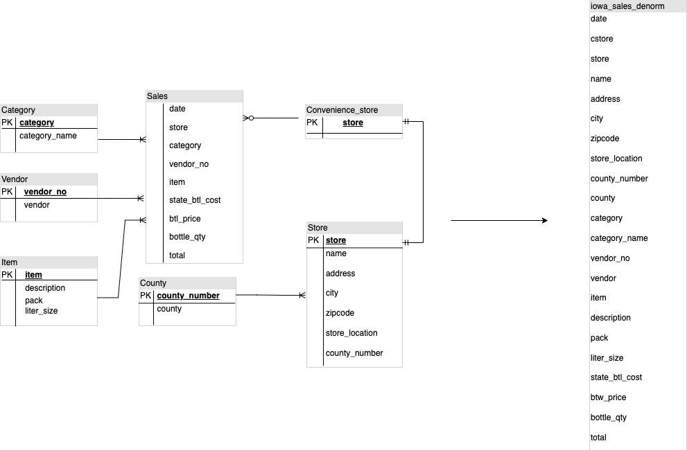
Techniques to flatten your existing schema
BigQuery technology leverages a combination of columnar data access and processing, in-memory storage, and distributed processing to provide quality query performance.
When designing a BigQuery DWH schema, creating a fact table in a
flat table structure (consolidating all the dimension tables into a single
record in the fact table) is better for storage utilization than using multiple
DWH dimensions tables. On top of less storage utilization, having a flat table
in BigQuery leads to less JOIN usage. The following diagram
illustrates an example of flattening your schema.
Example of flattening a star schema
Figure 1 shows a fictional sales management database that includes four tables:
- Orders/sales table (fact table)
- Employee table
- Location table
- Customer table
The primary key for the sales table is the OrderNum, which also contains
foreign keys to the other three tables.
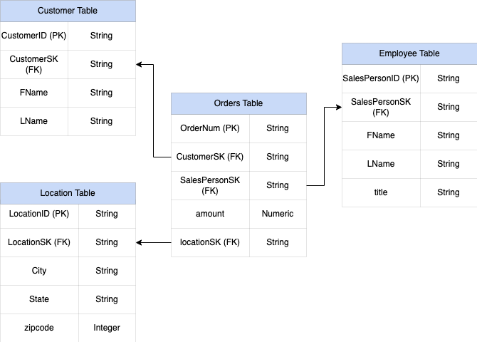
Figure 1: Sample sales data in a star schema
Sample data
Orders/fact table content
| OrderNum | CustomerID | SalesPersonID | amount | Location |
| O-1 | 1234 | 12 | 234.22 | 18 |
| O-2 | 4567 | 1 | 192.10 | 27 |
| O-3 | 12 | 14.66 | 18 | |
| O-4 | 4567 | 4 | 182.00 | 26 |
Employee table content
| SalesPersonID | FName | LName | title |
| 1 | Alex | Smith | Sales Associate |
| 4 | Lisa | Doe | Sales Associate |
| 12 | John | Doe | Sales Associate |
Customer table content
| CustomerID | FName | LName |
| 1234 | Amanda | Lee |
| 4567 | Matt | Ryan |
Location table content
| Location | city | city | city |
| 18 | Bronx | NY | 10452 |
| 26 | Mountain View | CA | 90210 |
| 27 | Chicago | IL | 60613 |
Query to flatten the data using LEFT OUTER JOIN
#standardSQL
INSERT INTO flattened
SELECT
  orders.ordernum,
  orders.customerID,
  customer.fname,
  customer.lname,
  orders.salespersonID,
  employee.fname,
  employee.lname,
  employee.title,
  orders.amount,
  orders.location,
  location.city,
  location.state,
  location.zipcode
FROM orders
LEFT OUTER JOIN customer
  ON customer.customerID = orders.customerID
LEFT OUTER JOIN employee
  ON employee.salespersonID = orders.salespersonID
LEFT OUTER JOIN location
  ON location.locationID = orders.locationID
Output of the flattened data
| OrderNum | CustomerID | FName | LName | SalesPersonID | FName | LName | amount | Location | city | state | zipcode |
| O-1 | 1234 | Amanda | Lee | 12 | John | Doe | 234.22 | 18 | Bronx | NY | 10452 |
| O-2 | 4567 | Matt | Ryan | 1 | Alex | Smith | 192.10 | 27 | Chicago | IL | 60613 |
| O-3 | 12 | John | Doe | 14.66 | 18 | Bronx | NY | 10452 | |||
| O-4 | 4567 | Matt | Ryan | 4 | Lisa | Doe | 182.00 | 26 | Mountain
View |
CA | 90210 |
Nested and repeated fields
In order to design and create a DWH schema from a relational schema (for example, star and snowflake schemas holding dimension and fact tables), BigQuery presents the nested and repeated fields functionality. Therefore, relationships can be preserved in a similar way as a relational normalized (or partial normalized) DWH schema without affecting the performance. For more information, see performance best practices.
To better understand the implementation of nested and repeated fields, look at a
simple relational schema of a CUSTOMERS table and ORDER/SALES table. They
are two different tables, one for each entity, and the relationships are defined
using a key such as a primary key and a foreign key as the link between the
tables while querying using JOINs. BigQuery nested and repeated
fields let you preserve the same relationship between the entities in one single
table. This can be implemented by having all the customer data, while the orders
data is nested for each of the customers. For more information, see Specifying
nested and repeated columns.
To convert the flat structure into a nested or repeated schema, nest the fields as follows:
CustomerID,FName,LNamenested into a new field calledCustomer.SalesPersonID,FName,LNamenested into a new field calledSalesperson.LocationID,city,state,zip codenested into a new field calledLocation.
Fields OrderNum and amount are not nested, as they represent unique
elements.
You want to make your schema flexible enough to allow for every order to have more than one customer: a primary and a secondary. The customer field is marked as repeated. The resulting schema is shown in Figure 2, which illustrates nested and repeated fields.
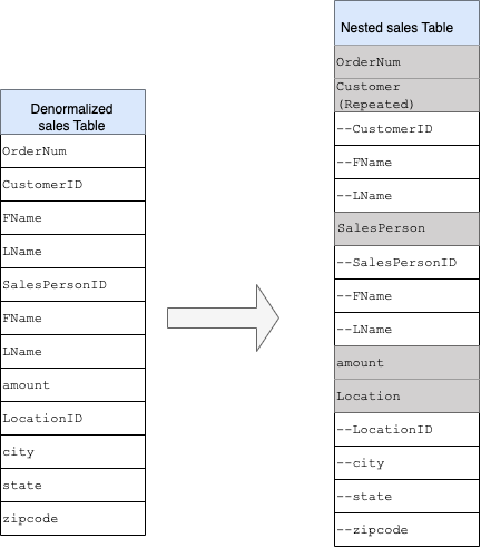
Figure 2: Logical representation of a nested structure
In some cases, denormalization using nested and repeated fields does not lead to performance improvements. For more information about limitations and restrictions, see Specify nested and repeated columns in table schemas.
Surrogate keys
It is common to identify rows with unique keys within the tables. Sequences are
commonly used at Oracle to create these keys. In
BigQuery you can create surrogate keys by using row_number and
partition by functions. For more information, see BigQuery and
surrogate keys: a practical
approach.
Keeping track of changes and history
When planning a BigQuery DWH migration, consider the concept of slowly changing dimensions (SCD). In general, the term SCD describes the process of making changes (DML operations) in the dimension tables.
For several reasons, traditional data warehouses use different types for handling data changes and keeping historical data in slowly changing dimensions. These type usages are needed by the hardware limitations and efficiency requirements discussed earlier. Because the storage is much cheaper than compute and infinitely scalable, data redundancy and duplication is encouraged if it results in faster queries in BigQuery. You can use data snapshotting techniques in which the whole data is loaded into new daily partitions.
Role-specific and user-specific views
Use role-specific and user-specific views when users belong to different teams and should see only records and results that they need.
BigQuery supports column- and row-level security. Column-level security provides fine-grained access to sensitive columns using policy tags, or type-based classification of data. Row-level security which lets you filter data and enables access to specific rows in a table based on qualifying user conditions.
Data migration
This section provides information about data migration from Oracle to BigQuery, including initial load, change data capture (CDC), and ETL/ELT tools and approaches.
Migration activities
It is recommended to perform migration in phases by identifying appropriate use cases for migration. There are multiple tools and services available to migrate data from Oracle to Google Cloud. While this list is not exhaustive, it does provide a sense of the size and scope of the migration effort.
Exporting data out of Oracle: For more information, see Initial load and CDC and streaming ingestion from Oracle to BigQuery. ETL tools can be used for the initial load.
Data staging (in Cloud Storage): Cloud Storage is the recommended landing place (staging area) for data exported from Oracle. Cloud Storage is designed for fast, flexible ingestion of structured or unstructured data.
ETL process: For more information, see ETL/ELT migration.
Loading data directly into BigQuery: You can load data into BigQuery directly from Cloud Storage, through Dataflow, or through real-time streaming. Use Dataflow when data transformation is required.
Initial load
Migration of the initial data from the existing Oracle data warehouse to BigQuery might be different from the incremental ETL/ELT pipelines depending on the data size and the network bandwidth. The same ETL/ELT pipelines, can be used if the data size is a couple of terabytes.
If the data is up to a few terabytes, dumping the data and using gcloud storage
for the transfer can be much more efficient than using JdbcIO-like programmatic database
extraction methodology, because programmatic approaches might need much more
granular performance tuning. If the data size is more than a few terabytes and
the data is stored in cloud or online storage (such as Amazon Simple Storage Service (Amazon S3)), consider
using BigQuery Data Transfer Service. For large-scale transfers
(especially transfers with limited network bandwidth), Transfer
Appliance is a useful option.
Constraints for initial load
When planning for data migration, consider the following:
- Oracle DWH data size: The source size of your schema carries a significant weight on the chosen data transfer method, especially when the data size is large (terabytes and above). When the data size is relatively small, the data transfer process can be completed in fewer steps. Dealing with large-scale data sizes makes the overall process more complex.
Downtime: Deciding whether downtime is an option for your migration to BigQuery is important. To reduce downtime, you can bulk load the steady historical data and have a CDC solution to catch up with changes that happen during the transfer process.
Pricing: In some scenarios, you might need third-party integration tools (for example, ETL or replication tools) that require additional licenses.
Initial data transfer (batch)
Data transfer using a batch method indicates that the data would be exported consistently in a single process (for example, exporting the Oracle DWH schema data into CSV, Avro, or Parquet files or importing to Cloud Storage to create datasets on BigQuery. All the ETL tools and concepts explained in ETL/ELT migration can be used for the initial load.
If you do not want to use an ETL/ELT tool for the initial load, you can write
custom scripts to export data to files (CSV, Avro, or Parquet) and upload that
data to Cloud Storage using gcloud storage, BigQuery Data Transfer Service, or
Transfer Appliance. For more information about performance tuning large data
transfers and transfer options, see Transferring your large data
sets. Then load data from
Cloud Storage to BigQuery.
Cloud Storage is ideal for handling the initial landing for data. Cloud Storage is a highly available and durable object storage service with no limitations on the number of files, and you pay only for the storage you use. The service is optimized to work with other Google Cloud services such as BigQuery and Dataflow.
CDC and streaming ingestion from Oracle to BigQuery
There are several ways to capture the changed data from Oracle. Each option has trade-offs, mainly in the performance impact on the source system, development and configuration requirements, and pricing and licensing.
Log-based CDC
Oracle GoldenGate is Oracle's recommended tool for extracting redo logs, and you can use GoldenGate for Big Data for streaming logs into BigQuery. GoldenGate requires per-CPU licensing. For information about the price, see Oracle Technology Global Price List. If Oracle GoldenGate for Big Data is available (in case licenses have already been acquired), using GoldenGate can be a good choice to create data pipelines to transfer data (initial load) and then sync all data modification.
Oracle XStream
Oracle stores every commit in redo log files, and these redo files can be used for CDC. Oracle XStream Out is built on top of LogMiner and provided by third-party tools such as Debezium (as of version 0.8) or commercially using tools such as Striim. Using XStream APIs requires purchasing a license for Oracle GoldenGate even if GoldenGate is not installed and used. XStream enables you to propagate Streams messages between Oracle and other software efficiently.
Oracle LogMiner
No special license is required for LogMiner. You can use the LogMiner option in the Debezium community connector. It is also available commercially using tools such as Attunity, Striim, or StreamSets. LogMiner might have some performance impact on a very active source database and should be used carefully in cases when the volume of changes (the size of the redo) is more than 10 GB per hour depending on the server's CPU, memory, and I/O capacity and utilization.
SQL-based CDC
This is the incremental ETL approach in which SQL queries continuously poll the
source tables for any changes depending on a monotonically increasing key and a
timestamp column that holds the last modified or inserted date. If there is no
monotonically increasing key, using the timestamp column (modified date) with a
small precision (seconds) can cause duplicate records or missed data depending
on the volume and comparison operator, such as > or >=.
To overcome such issues, you can use higher precision in timestamp columns such as six fractional digits (microseconds, which is the maximum supported precision in BigQuery, or you can add deduplication tasks in your ETL/ELT pipeline, depending on the business keys and data characteristics.
There should be an index on the key or timestamp column for better extract
performance and less impact on the source database. Delete operations are a
challenge for this methodology because they should be handled in the source
application in a soft delete way, such as puttint a deleted flag and updating
last_modified_date. An alternative solution can be logging these operations in
another table using a trigger.
Triggers
Database triggers can be created on source tables to log changes into shadow
journal tables. Journal tables can hold entire rows to keep track of every
column change, or they can only keep the primary key with the operation type
(insert, update, or delete). Then changed data can be captured with an SQL-based
approach described in SQL-based CDC. Using triggers can
affect the transaction performance and double the single-row DML operation
latency if a full row is stored. Storing only the primary key can reduce this
overhead, but in that case, a JOIN operation with the original table is
required in the SQL-based extraction, which misses the intermediate change.
ETL/ELT migration
There are many possibilities for handling ETL/ELT on Google Cloud. Technical guidance on specific ETL workload conversions is not in the scope of this document. You can consider a lift and shift approach or rearchitect your data integration platform depending on constraints such as cost and time. For more information about how to migrate your data pipelines to Google Cloud and many other migration concepts, see Migrate data pipelines.
Lift and shift approach
If your existing platform supports BigQuery and you want to continue using your existing data integration tool:
- You can keep the ETL/ELT platform as it is and change the necessary storage stages with BigQuery in your ETL/ELT jobs.
- If you want to migrate the ETL/ELT platform to Google Cloud as well, you can ask your vendor whether their tool is licensed on Google Cloud, and if it is, you can install it on Compute Engine or check the Google Cloud Marketplace.
For information about the data integration solution providers, see BigQuery partners.
Rearchitecting ETL/ELT platform
If you want to rearchitect your data pipelines, we recommend that you strongly consider using Google Cloud services.
Cloud Data Fusion
Cloud Data Fusion is a managed CDAP on Google Cloud offering a visual interface with many plugins for tasks such as drag-and-drop and pipeline developments. Cloud Data Fusion can be used for capturing data from many different kinds of source systems and offers batch and streaming replication capabilities. Cloud Data Fusion or Oracle plugins can be used to capture data from an Oracle. A BigQuery plugin can be used to load the data to BigQuery and handle schema updates.
No output schema is defined both on source and sink plugins, and
select * from is used in the source plugin to replicate new columns as well.
You can use the Cloud Data Fusion Wrangle feature for data cleaning and preparing.
Dataflow
Dataflow is a serverless data processing platform that can autoscale as well as do batch and streaming data processing. Dataflow can be a good choice for Python and Java developers who want to code their data pipelines and use the same code for both streaming and batch workloads. Use the JDBC to BigQuery template to extract data from your Oracle or other relational databases and load it into BigQuery.
Cloud Composer
Cloud Composer is Google Cloud fully managed workflow orchestration service built on Apache Airflow. It lets you author, schedule, and monitor pipelines that span across cloud environments and on-premises data centers. Cloud Composer provides operators and contributions that can run multi-cloud technologies for use cases including extract and loads, transformations of ELT, and REST API calls.
Cloud Composer uses directed acyclic graphs (DAGs) for scheduling and orchestrating workflows. To understand the general airflow concepts, see Airflow Apache concepts. For more information about DAGs, see Writing DAGs (workflows). For sample ETL best practices with Apache Airflow, see ETL best practices with Airflow documentation site¶. You can replace the Hive operator in that example with the BigQuery operator, and the same concepts would be applicable.
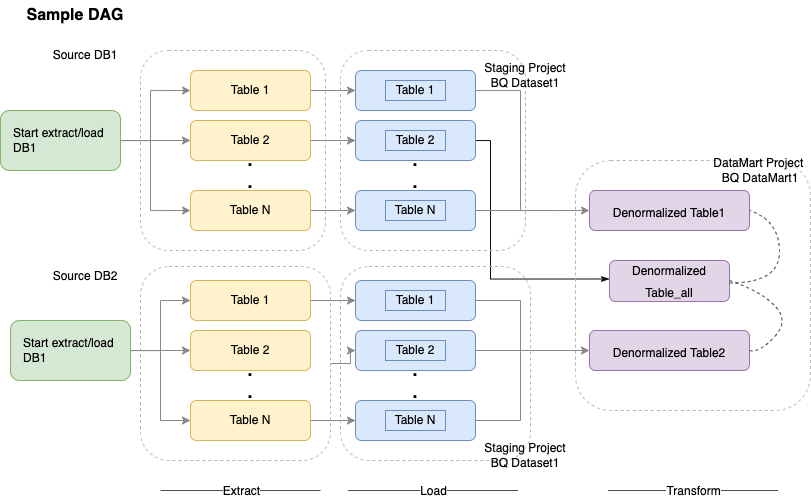
The following sample code is a high-level part of a sample DAG for the preceding diagram:
    default_args = {
      'owner': 'airflow',
      'depends_on_past': False,
     'start_date': airflow.utils.dates.days_ago(2),
     'email': ['airflow@example.com'],
     'email_on_failure': False,
     'email_on_retry': False,
     'retries': 2,
     'retry_delay': timedelta(minutes=10),
    }
    schedule_interval = "00 01 * * *"
    dag = DAG('load_db1_db2',catchup=False, default_args=default_args,
    schedule_interval=schedule_interval)
    tables = {
      'DB1_TABLE1': {'database':'DB1', 'table_name':'TABLE1'},
      'DB1_TABLE2': {'database':'DB1', 'table_name':'TABLE2'},
      'DB1_TABLEN': {'database':'DB1', 'table_name':'TABLEN'},
      'DB2_TABLE1': {'database':'DB2', 'table_name':'TABLE1'},
      'DB2_TABLE2': {'database':'DB2', 'table_name':'TABLE2'},
      'DB2_TABLEN': {'database':'DB2', 'table_name':'TABLEN'},
    }
    start_db1_daily_incremental_load = DummyOperator(
       task_id='start_db1_daily_incremental_load', dag=dag)
    start_db2_daily_incremental_load = DummyOperator(
       task_id='start_db2_daily_incremental_load', dag=dag)

    load_denormalized_table1 = BigQueryOperator(
       task_id='load_denormalized_table1',
       use_legacy_sql=False,
       write_disposition='WRITE_TRUNCATE',
       allow_large_results=True,
       trigger_rule='all_done',
       bql='''
       #standardSQL
       select
           t1.*,tN.* except (ID)
           from `ingest-project.ingest_db1.TABLE1` as t1
           left join `ingest-project.ingest_db1.TABLEN` as tN on t1.ID = tN.ID
        ''',    destination_dataset_table='datamart-project.dm1.dt1', dag=dag)

        load_denormalized_table2 = BigQueryOperator(
           task_id='load_denormalized_table2',
           use_legacy_sql=False,
           write_disposition='WRITE_TRUNCATE',
           allow_large_results=True,
           trigger_rule='all_done',
        bql='''
        #standardSQL
        select
           t1.*,t2.* except (ID),tN.* except (ID)
           from `ingest-project.ingest_db1.TABLE1` as t1
           left join `ingest-project.ingest_db2.TABLE2` as t2 on t1.ID = t2.ID
           left join `ingest-project.ingest_db2.TABLEN` as tN on t2.ID = tN.ID
        ''',    destination_dataset_table='datamart-project.dm1.dt2', dag=dag)

        load_denormalized_table_all = BigQueryOperator(
           task_id='load_denormalized_table_all',
           use_legacy_sql=False,
           write_disposition='WRITE_TRUNCATE',
           allow_large_results=True,
          trigger_rule='all_done',
        bql='''
        #standardSQL
        select
           t1.*,t2.* except (ID),t3.* except (ID)
           from `datamart-project.dm1.dt1` as t1
           left join `ingest-project.ingest_db1.TABLE2` as t2 on t1.ID = t2.ID
           left join `datamart-project.dm1.dt2` as t3 on t2.ID = t3.ID
        ''',    destination_dataset_table='datamart-project.dm1.dt_all', dag=dag)

        def start_pipeline(database,table,...):
        #start initial or incremental load job here
        #you can write your custom operator to integrate ingestion tool
        #or you can use operators available in composer instead

        for table,table_attr in tables.items():
        tbl=table_attr['table_name']
        db=table_attr['database'])
        load_start = PythonOperator(
        task_id='start_load_{db}_{tbl}'.format(tbl=tbl,db=db),
        python_callable=start_pipeline,
        op_kwargs={'database': db,
        'table':tbl},
        dag=dag
        )

        load_monitor = HttpSensor(
          task_id='load_monitor_{db}_{tbl}'.format(tbl=tbl,db=db),
          http_conn_id='ingestion-tool',
          endpoint='restapi-endpoint/',
          request_params={},
          response_check=lambda response: """{"status":"STOPPED"}""" in
          response.text,
          poke_interval=1,
          dag=dag,
        )

        load_start.set_downstream(load_monitor)

        if table_attr['database']=='db1':
          load_start.set_upstream(start_db1_daily_incremental_load)
        else:
          load_start.set_upstream(start_db2_daily_incremental_load)

        if table_attr['database']=='db1':
          load_monitor.set_downstream(load_denormalized_table1)
        else:
          load_monitor.set_downstream(load_denormalized_table2)
          load_denormalized_table1.set_downstream(load_denormalized_table_all)
          load_denormalized_table2.set_downstream(load_denormalized_table_all)
The preceding code is provided for demonstration purposes and cannot be used as it is.
Dataprep by Trifacta
Dataprep is a data service for visually exploring, cleaning, and preparing structured and unstructured data for analysis, reporting, and machine learning. You export the source data into JSON or CSV files, transform the data using Dataprep, and load the data using Dataflow. For an example, see Oracle data (ETL) to BigQuery using Dataflow and Dataprep.
Dataproc
Dataproc is a Google managed Hadoop service. You
can use Sqoop to export data from Oracle and many relational databases into
Cloud Storage as Avro files, and then you can load Avro files into
BigQuery using the bq tool. It
is very common to install ETL tools like CDAP on Hadoop that use JDBC to extract
data and Apache Spark or MapReduce for transformations of the data.
Partner tools for data migration
There are several vendors in the extraction, transformation, and load (ETL) space. ETL market leaders such as Informatica, Talend, Matillion, Infoworks, Stitch, Fivetran, and Striim have deeply integrated with both BigQuery and Oracle and can help extract, transform, load data, and manage processing workflows.
ETL tools have been around for many years. Some organizations might find it convenient to leverage an existing investment in trusted ETL scripts. Some of our key partner solutions are included on BigQuery partner website. Knowing when to choose partner tools over Google Cloud built-in utilities depends on your current infrastructure and your IT team's comfort with developing data pipelines in Java or Python code.
Business intelligence (BI) tool migration
BigQuery supports a flexible suite of business intelligence (BI) solutions for Reporting and analysis that you can leverage. For more information about BI tool migration and BigQuery integration, see Overview of BigQuery analytics.
Query (SQL) translation
BigQuery's GoogleSQL supports compliance with the SQL 2011 standard and has extensions that support querying nested and repeated data. All ANSI-compliant SQL functions and operators can be used with minimal modifications. For a detailed comparison between Oracle and BigQuery SQL syntax and functions, see the Oracle to BigQuery SQL translation reference.
Use batch SQL translation to migrate your SQL code in bulk, or interactive SQL translation to translate ad hoc queries.
Migrating Oracle options
This section presents architectural recommendations and references for converting applications that use Oracle Data Mining, R, and Spatial and Graph functionalities.
Oracle Advanced Analytics option
Oracle offers advanced analytics options for data mining, fundamental machine learning (ML) algorithms, and R usage. The Advanced Analytics option requires licensing. You can choose from a comprehensive list of Google AI/ML products depending on your needs from development to production at scale.
Oracle R Enterprise
Oracle R Enterprise (ORE), a component of the Oracle Advanced Analytics option, makes the open source R statistical programming language integrate with Oracle Database. In standard ORE deployments, R is installed on an Oracle server.
For very large scales of data or approaches to warehousing, integrating R with BigQuery is an ideal choice. You can use the open source bigrquery R library to integrate R with BigQuery.
Google has partnered with RStudio to make the field's cutting-edge tools available to users. RStudio can be used to access terabytes of data in BigQuery fit models in TensorFlow, and run machine learning models at scale with AI Platform. In Google Cloud, R can be installed on Compute Engine at scale.
Oracle Data Mining
Oracle Data Mining (ODM), a component of the Oracle Advanced Analytics option, lets developers build machine learning models using Oracle PL/SQL Developer on Oracle.
BigQuery ML enables developers to run many different types of models, such as linear regression, binary logistic regression, multiclass logistic regression, k-means clustering, and TensorFlow model imports. For more information, see Introduction to BigQuery ML.
Converting ODM jobs might require rewriting the code. You can choose from comprehensive Google AI product offerings such as BigQuery ML, AI APIs (Speech-to-Text, Text-to-Speech, Dialogflow, Cloud Translation, Cloud Natural Language API, Cloud Vision, Timeseries Insights API, and more), or Vertex AI.
Vertex AI Workbench can be used as a development environment for data scientists, and Vertex AI Training can be used to run training and scoring workloads at scale.
Spatial and Graph option
Oracle offers the Spatial and Graph option for querying geometry and graphs and requires licensing for this option. You can use the geometry functions in BigQuery without additional costs or licenses and use other graph databases in Google Cloud.
Spatial
BigQuery offers geospatial analytics functions and data types. For more information, see Working with geospatial analytics data. Oracle Spatial data types and functions can be converted to geography functions in BigQuery standard SQL. Geography functions don't add cost on top of standard BigQuery pricing.
Graph
JanusGraph is an open source graph database solution that can use Bigtable as a storage backend. For more information, see Running JanusGraph on GKE with Bigtable.
Neo4j is another graph database solution delivered as a Google Cloud service that runs on Google Kubernetes Engine (GKE).
Oracle Application Express
Oracle Application Express (APEX) applications are unique to Oracle and need to be rewritten. Reporting and data visualization functionalities can be developed using Looker Studio or BI engine, whereas application-level functionalities such as creating and editing rows can be developed without coding on AppSheet using Cloud SQL.
What's next
- Learn how to Optimize workloads for overall performance optimization and cost reduction.
- Learn about how to Optimize storage in BigQuery.
- For BigQuery updates, see release notes.
- Reference the Oracle SQL translation guide.