Overview of BigQuery storage

This page describes the storage component of BigQuery.

BigQuery storage is optimized for running analytic queries over large datasets. It also supports high-throughput streaming ingestion and high-throughput reads. Understanding BigQuery storage can help you to optimize your workloads.

Overview

One of the key features of BigQuery's architecture is the separation of storage and compute. This allows BigQuery to scale both storage and compute independently, based on demand.

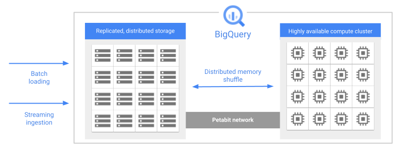
When you run a query, the query engine distributes the work in parallel across multiple workers, which scan the relevant tables in storage, process the query, and then gather the results. BigQuery executes queries completely in memory, using a petabit network to ensure that data moves extremely quickly to the worker nodes.

Here are some key features of BigQuery storage:

Managed. BigQuery storage is a completely managed service. You don't need to provision storage resources or reserve units of storage. BigQuery automatically allocates storage for you when you load data into the system. You only pay for the amount of storage that you use. The BigQuery pricing model charges for compute and storage separately. For pricing details, see BigQuery pricing.
Durable. BigQuery storage is designed for 99.999999999% (11 9's) annual durability. BigQuery replicates your data across multiple availability zones to protect from data loss due to machine-level failures or zonal failures. For more information, see Reliability: Disaster planning.
Encrypted. BigQuery automatically encrypts all data before it is written to disk. You can provide your own encryption key or let Google manage the encryption key. For more information, see Encryption at rest.
Efficient. BigQuery storage uses an efficient encoding format that is optimized for analytic workloads. If you want to learn more about BigQuery's storage format, see the blog post Inside Capacitor, BigQuery's next-generation columnar storage format.

Table data

The majority of the data that you store in BigQuery is table data. Table data includes standard tables, table clones, table snapshots, and materialized views. You are billed for the storage that you use for these resources.

Standard tables contain structured data. Every table has a schema, and every column in the schema has a data type. BigQuery stores data in columnar format. See Storage layout in this document.
Table clones are lightweight, writable copies of standard tables. BigQuery only stores the delta between a table clone and its base table.
Table snapshots are point-in-time copies of tables. Table snapshots are read-only, but you can restore a table from a table snapshot. BigQuery only stores the delta between a table snapshot and its base table.
Materialized views are precomputed views that periodically cache the results of the view query. The cached results are stored in BigQuery storage.

In addition, cached query results are stored as temporary tables. You aren't charged for cached query results stored in temporary tables.

External tables are a special type of table, where the data resides in a data store that is external to BigQuery, such as Cloud Storage. An external table has a table schema, just like a standard table, but the table definition points to the external data store. In this case, only the table metadata is kept in BigQuery storage. BigQuery does not charge for external table storage, although the external data store might charge for storage.

BigQuery organizes tables and other resources into logical containers called datasets. How you group your BigQuery resources affects permissions, quotas, billing, and other aspects of your BigQuery workloads. For more information and best practices, see Organizing BigQuery resources.

Metadata

BigQuery storage also holds metadata about your BigQuery resources. You aren't charged for metadata storage.

When you create any persistent entity in BigQuery, such as a table, view, or user-defined function (UDF), BigQuery stores metadata about the entity. This is true even for resources that don't contain any table data, such as UDFs and logical views.

Metadata includes information such as the table schema, partitioning and clustering specifications, table expiration times, and other information. This type of metadata is visible to the user and can be configured when you create the resource. In addition, BigQuery stores metadata that it uses internally to optimize queries. This metadata is not directly visible to users.

Storage layout

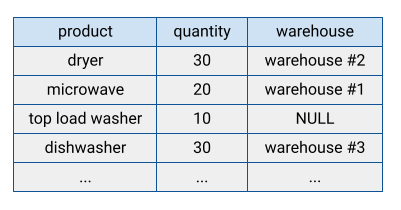
Many traditional database systems store their data in row-oriented format, meaning rows are stored together, with the fields in each row appearing sequentially on disk. Row-oriented databases are efficient at looking up individual records. However, they can be less efficient at performing analytical functions across many records, because the system has to read every field when accessing a record.

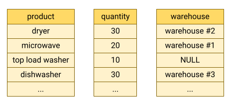
BigQuery stores table data in columnar format, meaning it stores each column separately. Column-oriented databases are particularly efficient at scanning individual columns over an entire dataset.

Column-oriented databases are optimized for analytic workloads that aggregate data over a very large number of records. Often, an analytic query only needs to read a few columns from a table. For example, if you want to compute the sum of a column over millions of rows, BigQuery can read that column data without reading every field of every row.

Another advantage of column-oriented databases is that data within a column typically has more redundancy than data across a row. This characteristic allows for greater data compression by using techniques such as run-length encoding, which can improve read performance.

BigQuery does not support foreign keys. This makes BigQuery more suitable for OLAP and data warehouse workloads than OLTP workloads. For OLTP workloads, consider using either Cloud Spanner or Cloud SQL. BigQuery supports federated queries with both of these database services.

Optimize storage

Optimizing BigQuery storage improves query performance and controls cost. To view the table storage metadata, query the following INFORMATION_SCHEMA views:

For information about optimizing storage, see Optimize storage in BigQuery.

Load data

There are several basic patterns for ingesting data into BigQuery.

Batch load: Load your source data into a BigQuery table in a single batch operation. This can be a one-time operation or you can automate it to occur on a schedule. A batch load operation can create a new table or append data into an existing table.
Streaming: Continually stream smaller batches of data, so that the data is available for querying in near-real-time.
Generated data: Use SQL statements to insert rows into an existing table or write the results of a query to a table.

For more information about when to choose each of these ingestion methods, see Introduction to loading data. For pricing information, see Data ingestion pricing.

Read data from BigQuery storage

Most of the time, you store data in BigQuery in order to run analytical queries on that data. However, sometimes you might want to read records directly from a table. BigQuery provides several ways to read table data:

BigQuery API: Synchronous paginated access with the tabledata.list method. Data is read in a serial fashion, one page per invocation. For more information, see Browsing table data.
BigQuery Storage API: Streaming high-throughput access that also supports server-side column projection and filtering. Reads can be parallelized across many readers by segmenting them into multiple disjoint streams.
Export: Asynchronous high-throughput copying to Google Cloud Storage, either with extract jobs or the EXPORT DATA. If you need to copy data in Cloud Storage, export the data either with an extract job or an EXPORT DATA statement.
Copy: Asynchronous copying of datasets within BigQuery. The copy is done logically when the source and destination location is the same.

For pricing information, see Data extraction pricing.

Based on the application requirements, you can read the table data:

Read and copy: If you need an at-rest copy in Cloud Storage, export the data either with an extract job or an EXPORT DATA statement. If you only want to read the data, use the BigQuery Storage API. If you want to make a copy within BigQuery, then use a copy job.
Scale: The BigQuery API is the least efficient method and shouldn't be used for high volume reads. If you need to export more than 50 TB of data per day, use the EXPORT DATA statement or the BigQuery Storage API.
Time to return the first row: The BigQuery API is the fastest method to return the first row, but should only be used to read small amounts of data. The BigQuery Storage API is slower to return the first row, but has much higher-throughput. Exports and copies must finish before any rows can be read, so the time to the first row for these types of jobs can be on the order of minutes.

Deletion

When you delete a table, the data persists for at least the duration of your time travel window. After this, data is cleaned up from disk within the Google Cloud deletion timeline. Some deletion operations, such as the DROP COLUMN statement, are metadata-only operations. In this case, storage is freed up the next time you modify the affected rows. If you do not modify the table, there is no guaranteed time within which the storage is freed up. For more information, see Data deletion on Google Cloud.

What's next

Learn about working with tables.
Learn how to optimize storage.
Learn how to query data in BigQuery.
Learn about data security and governance.