This tutorial teaches you how to use an
ARIMA_PLUS univariate time series model to forecast the future value of a given
column, based on the historical values for that column.
This tutorial forecasts for multiple time series. Forecasted values are calculated for each time point, for each value in one or more specified columns. For example, if you wanted to forecast weather and specified a column containing city data, the forecasted data would contain forecasts for all time points for City A, then forecasted values for all time points for City B, and so forth.
This tutorial uses data from the public
bigquery-public-data.new_york.citibike_trips
table. This table contains information about Citi Bike trips in New York City.
Before reading this tutorial, we highly recommend that you read Forecast a single time series with a univariate model.
Objectives
This tutorial guides you through completing the following tasks:
- Creating a time series model to forecast the number of bike trips by using the
CREATE MODELstatement. - Evaluating the autoregressive integrated moving average (ARIMA) information
in the model by using the
ML.ARIMA_EVALUATEfunction. - Inspecting the model coefficients by using the
ML.ARIMA_COEFFICIENTSfunction. - Retrieving the forecasted bike ride information from the model by using the
ML.FORECASTfunction. - Retrieving components of the time series, such as seasonality and trend,
by using the
ML.EXPLAIN_FORECASTfunction. You can inspect these time series components in order to explain the forecasted values.
Costs
This tutorial uses billable components of Google Cloud, including:
- BigQuery
- BigQuery ML
For more information about BigQuery costs, see the BigQuery pricing page.
For more information about BigQuery ML costs, see BigQuery ML pricing.
Before you begin
- Sign in to your Google Cloud account. If you're new to Google Cloud, create an account to evaluate how our products perform in real-world scenarios. New customers also get $300 in free credits to run, test, and deploy workloads.
-
In the Google Cloud console, on the project selector page, select or create a Google Cloud project.
-
Verify that billing is enabled for your Google Cloud project.
-
In the Google Cloud console, on the project selector page, select or create a Google Cloud project.
-
Verify that billing is enabled for your Google Cloud project.
- BigQuery is automatically enabled in new projects.
To activate BigQuery in a pre-existing project, go to
Enable the BigQuery API.
Required Permissions
To create the dataset, you need the
bigquery.datasets.createIAM permission.To create the model, you need the following permissions:
bigquery.jobs.createbigquery.models.createbigquery.models.getDatabigquery.models.updateData
To run inference, you need the following permissions:
bigquery.models.getDatabigquery.jobs.create
For more information about IAM roles and permissions in BigQuery, see Introduction to IAM.
Create a dataset
Create a BigQuery dataset to store your ML model.
Console
In the Google Cloud console, go to the BigQuery page.
In the Explorer pane, click your project name.
Click View actions > Create dataset
On the Create dataset page, do the following:
For Dataset ID, enter
bqml_tutorial.For Location type, select Multi-region, and then select US (multiple regions in United States).
Leave the remaining default settings as they are, and click Create dataset.
bq
To create a new dataset, use the
bq mk command
with the --location flag. For a full list of possible parameters, see the
bq mk --dataset command
reference.
Create a dataset named
bqml_tutorialwith the data location set toUSand a description ofBigQuery ML tutorial dataset:bq --location=US mk -d \ --description "BigQuery ML tutorial dataset." \ bqml_tutorial
Instead of using the
--datasetflag, the command uses the-dshortcut. If you omit-dand--dataset, the command defaults to creating a dataset.Confirm that the dataset was created:
bq ls
API
Call the datasets.insert
method with a defined dataset resource.
{
  "datasetReference": {
     "datasetId": "bqml_tutorial"
  }
}
BigQuery DataFrames
Before trying this sample, follow the BigQuery DataFrames setup instructions in the BigQuery quickstart using BigQuery DataFrames. For more information, see the BigQuery DataFrames reference documentation.
To authenticate to BigQuery, set up Application Default Credentials. For more information, see Set up ADC for a local development environment.
Visualize the input data
Before creating the model, you can optionally visualize your input time series data to get a sense of the distribution. You can do this by using Looker Studio.
SQL
The SELECT statement of the following query uses the
EXTRACT function
to extract the date information from the starttime column. The query uses
the COUNT(*) clause to get the daily total number of Citi Bike trips.
Follow these steps to visualize the time series data:
In the Google Cloud console, go to the BigQuery page.
In the query editor, paste in the following query and click Run:
SELECT
 EXTRACT(DATE from starttime) AS date,
 COUNT(*) AS num_trips
FROM
`bigquery-public-data.new_york.citibike_trips`
GROUP BY date;
When the query completes, click Explore data > Explore with Looker Studio. Looker Studio opens in a new tab. Complete the following steps in the new tab.
In the Looker Studio, click Insert > Time series chart.
In the Chart pane, choose the Setup tab.
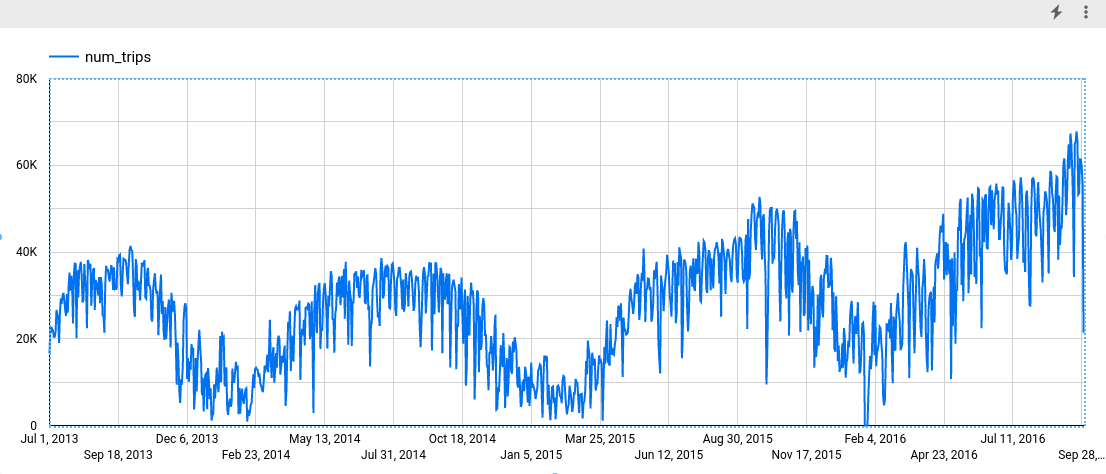
In the Metric section, add the num_trips field, and remove the default Record Count metric. The resulting chart looks similar to the following:
BigQuery DataFrames
Before trying this sample, follow the BigQuery DataFrames setup instructions in the BigQuery quickstart using BigQuery DataFrames. For more information, see the BigQuery DataFrames reference documentation.
To authenticate to BigQuery, set up Application Default Credentials. For more information, see Set up ADC for a local development environment.
Create the time series model
You want to forecast the number of bike trips for each Citi Bike station, which requires many time series models; one for each Citi Bike station that is included in the input data. You can create multiple models to do this, but that can be a tedious and time consuming process, especially when you have a large number of time series. Instead, you can use a single query to create and fit a set of time series models in order to forecast multiple time series at once.
SQL
In the following query, the
OPTIONS(model_type='ARIMA_PLUS', time_series_timestamp_col='date', ...)
clause indicates that you are creating an
ARIMA-based
time series model. You use the
time_series_id_col option
of the CREATE MODEL statement to specify one or more columns in the input data
that you want to get forecasts for, in this case the Citi Bike station, as
represented by the start_station_name column. You use the WHERE clause to
limit the start stations to those with Central Park in their names. The
auto_arima_max_order option
of the CREATE MODEL statement controls the
search space for hyperparameter tuning in the auto.ARIMA algorithm. The
decompose_time_series option
of the CREATE MODEL statement defaults to TRUE, so that information about
the time series data is returned when you evaluate the model in the next step.
Follow these steps to create the model:
In the Google Cloud console, go to the BigQuery page.
In the query editor, paste in the following query and click Run:
CREATE OR REPLACE MODEL `bqml_tutorial.nyc_citibike_arima_model_group`
OPTIONS
(model_type = 'ARIMA_PLUS',
 time_series_timestamp_col = 'date',
 time_series_data_col = 'num_trips',
 time_series_id_col = 'start_station_name',
 auto_arima_max_order = 5
) AS
SELECT
 start_station_name,
 EXTRACT(DATE from starttime) AS date,
 COUNT(*) AS num_trips
FROM
`bigquery-public-data.new_york.citibike_trips`
WHERE start_station_name LIKE '%Central Park%'
GROUP BY start_station_name, date;
The query takes approximately 24 seconds to complete, after which the
nyc_citibike_arima_model_groupmodel appears in the Explorer pane. Because the query uses aCREATE MODELstatement, you don't see query results.
This query creates twelve time series models, one for each of the twelve
Citi Bike start stations in the input data. The time cost, approximately 24
seconds, is only 1.4 times more than that of creating a single time series
model because of the parallelism. However, if you remove the
WHERE ... LIKE ... clause, there would be 600+ time series to forecast, and
they wouldn't be forecast completely in parallel because of slot capacity
limitations. In that case, the query would take approximately 15 minutes to
finish. To reduce the query runtime with the compromise of a potential slight
drop in model quality, you could decrease the value of the
auto_arima_max_order.
This shrinks the search space of hyperparameter tuning in the auto.ARIMA
algorithm. For more information, see
Large-scale time series forecasting best practices.
BigQuery DataFrames
In the following snippet, you are creating an ARIMA-based time series model.
Before trying this sample, follow the BigQuery DataFrames setup instructions in the BigQuery quickstart using BigQuery DataFrames. For more information, see the BigQuery DataFrames reference documentation.
To authenticate to BigQuery, set up Application Default Credentials. For more information, see Set up ADC for a local development environment.
This creates twelve time series models, one for each of the twelve Citi Bike start stations in the input data. The time cost, approximately 24 seconds, is only 1.4 times more than that of creating a single time series model because of the parallelism.
Evaluate the model
SQL
Evaluate the time series model by using the ML.ARIMA_EVALUATE
function. The ML.ARIMA_EVALUATE function shows you the evaluation metrics that
were generated for the model during the process of automatic
hyperparameter tuning.
Follow these steps to evaluate the model:
In the Google Cloud console, go to the BigQuery page.
In the query editor, paste in the following query and click Run:
SELECT
*
FROM
ML.ARIMA_EVALUATE(MODEL `bqml_tutorial.nyc_citibike_arima_model_group`);
The results should look like the following:
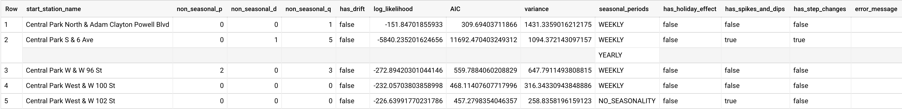
While
auto.ARIMAevaluates dozens of candidate ARIMA models for each time series,ML.ARIMA_EVALUATEby default only outputs the information of the best model to make the output table compact. To view all the candidate models, you can set theML.ARIMA_EVALUATEfunction'sshow_all_candidate_modelargument toTRUE.
BigQuery DataFrames
Before trying this sample, follow the BigQuery DataFrames setup instructions in the BigQuery quickstart using BigQuery DataFrames. For more information, see the BigQuery DataFrames reference documentation.
To authenticate to BigQuery, set up Application Default Credentials. For more information, see Set up ADC for a local development environment.
The start_station_name column identifies the input data column for which
time series were created. This is the column that you specified with the
time_series_id_col option when creating the model.
The non_seasonal_p, non_seasonal_d, non_seasonal_q, and has_drift
output columns define an ARIMA model in the training pipeline. The
log_likelihood, AIC, and varianceoutput columns are relevant to the ARIMA
model fitting process.The fitting process determines the best ARIMA model by
using the auto.ARIMA algorithm, one for each time series.
The auto.ARIMA algorithm uses the
KPSS test to determine the best value
for non_seasonal_d, which in this case is 1. When non_seasonal_d is 1,
the auto.ARIMA algorithm trains 42 different candidate ARIMA models in parallel.
In this example, all 42 candidate models are valid, so the output contains 42
rows, one for each candidate ARIMA model; in cases where some of the models
aren't valid, they are excluded from the output. These candidate models are
returned in ascending order by AIC. The model in the first row has the lowest
AIC, and is considered as the best model. This best model is saved as the final
model and is used when you forecast data, evaluate the model, and
inspect the model's coefficients as shown in the following steps.
The seasonal_periods column contains information about the seasonal pattern
identified in the time series data. Each time series can have different seasonal
patterns. For example, from the figure, you can see that one time series has a
yearly pattern, while others don't.
The has_holiday_effect, has_spikes_and_dips, and has_step_changes columns
are only populated when decompose_time_series=TRUE. These columns also reflect
information about the input time series data, and are not related to the ARIMA
modeling. These columns also have the same values across all output rows.
Inspect the model's coefficients
SQL
Inspect the time series model's coefficients by using the
ML.ARIMA_COEFFICIENTS function.
Follow these steps to retrieve the model's coefficients:
In the Google Cloud console, go to the BigQuery page.
In the query editor, paste in the following query and click Run:
SELECT
*
FROM
ML.ARIMA_COEFFICIENTS(MODEL `bqml_tutorial.nyc_citibike_arima_model_group`);
The query takes less than a second to complete. The results should look similar to the following:
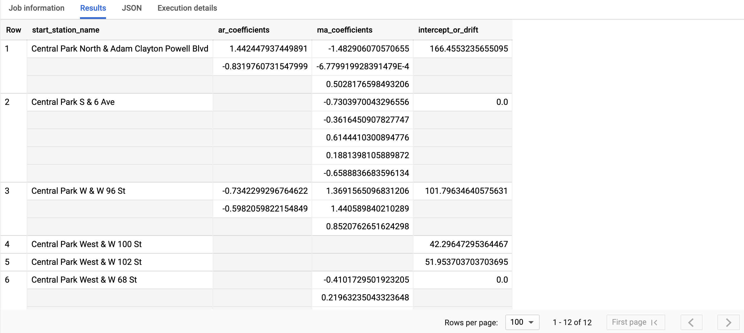
For more information about the output columns, see
ML.ARIMA_COEFFICIENTSfunction.
BigQuery DataFrames
Inspect the time series model's coefficients by using the
coef_ function.
Before trying this sample, follow the BigQuery DataFrames setup instructions in the BigQuery quickstart using BigQuery DataFrames. For more information, see the BigQuery DataFrames reference documentation.
To authenticate to BigQuery, set up Application Default Credentials. For more information, see Set up ADC for a local development environment.
The start_station_name column identifies the input data column for which
time series were created. This is the column that you specified in the
time_series_id_col option when creating the model.
The ar_coefficients output column shows the model coefficients of the
autoregressive (AR) part of the ARIMA model. Similarly, the ma_coefficients
output column shows the model coefficients of the moving-average (MA) part of
the ARIMA model. Both of these columns contain array values, whose lengths are
equal to non_seasonal_p and non_seasonal_q, respectively. The
intercept_or_drift value is the constant term in the ARIMA model.
Use the model to forecast data
SQL
Forecast future time series values by using the ML.FORECAST
function.
In the following GoogleSQL query, the
STRUCT(3 AS horizon, 0.9 AS confidence_level) clause indicates that the
query forecasts 3 future time points, and generates a prediction interval
with a 90% confidence level.
Follow these steps to forecast data with the model:
In the Google Cloud console, go to the BigQuery page.
In the query editor, paste in the following query and click Run:
SELECT
*
FROM
ML.FORECAST(MODEL `bqml_tutorial.nyc_citibike_arima_model_group`,
 STRUCT(3 AS horizon, 0.9 AS confidence_level))
Click Run.
The query takes less than a second to complete. The results should look like the following:
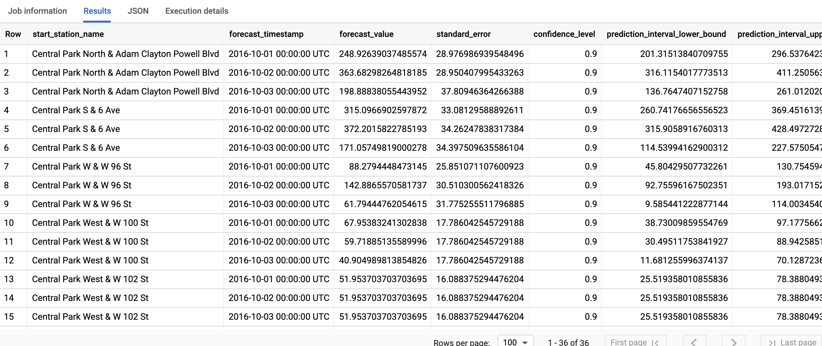
For more information about the output columns, see
ML.FORECAST function.
BigQuery DataFrames
Forecast future time series values by using the
predict function.
Before trying this sample, follow the BigQuery DataFrames setup instructions in the BigQuery quickstart using BigQuery DataFrames. For more information, see the BigQuery DataFrames reference documentation.
To authenticate to BigQuery, set up Application Default Credentials. For more information, see Set up ADC for a local development environment.
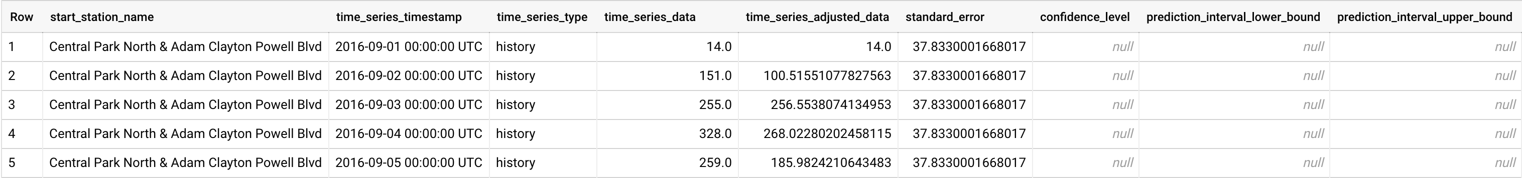
The first column, start_station_name, annotates the time series that each
time series model is fitted against. Each start_station_name has three
rows of forecasted results, as specified by the horizon value.
For each start_station_name, the output rows are in chronological order by the
forecast_timestamp column value. In time series forecasting, the prediction
interval, as represented by the prediction_interval_lower_bound and
prediction_interval_upper_bound column values, is as important as the
forecast_value column value. The forecast_value value is the middle point
of the prediction interval. The prediction interval depends on the
standard_error and confidence_level column values.
Explain the forecasting results
SQL
You can get explainability metrics in addition to forecast data by using the
ML.EXPLAIN_FORECAST function. The ML.EXPLAIN_FORECAST function forecasts
future time series values and also returns all the separate components of the
time series. If you just want to return forecast data, use the ML.FORECAST
function instead, as shown in
Use the model to forecast data.
The STRUCT(3 AS horizon, 0.9 AS confidence_level) clause used in the
ML.EXPLAIN_FORECAST function indicates that the query forecasts 3 future
time points and generates a prediction interval with 90% confidence.
Follow these steps to explain the model's results:
In the Google Cloud console, go to the BigQuery page.
In the query editor, paste in the following query and click Run:
SELECT
*
FROM
ML.EXPLAIN_FORECAST(MODEL `bqml_tutorial.nyc_citibike_arima_model_group`,
 STRUCT(3 AS horizon, 0.9 AS confidence_level));
The query takes less than a second to complete. The results should look like the following:
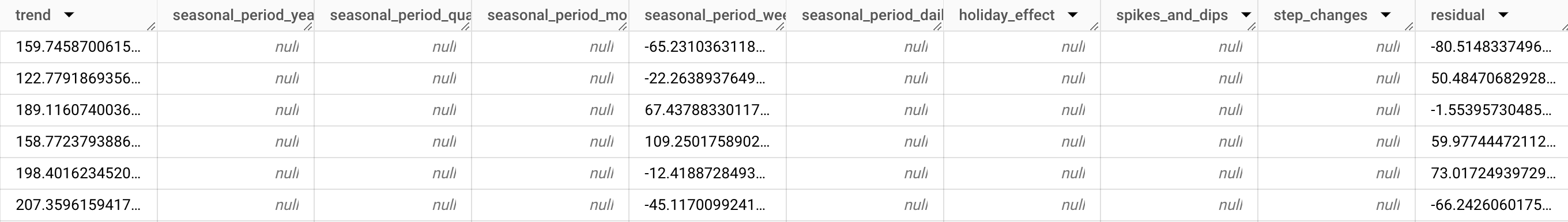
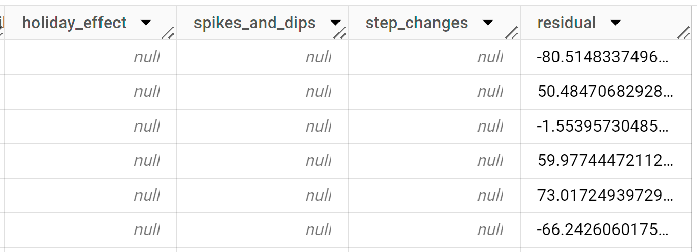
The first thousands rows returned are all history data. You must scroll through the results to see the forecast data.
The output rows are ordered first by
start_station_name, then chronologically by thetime_series_timestampcolumn value. In time series forecasting, the prediction interval, as represented by theprediction_interval_lower_boundandprediction_interval_upper_boundcolumn values, is as important as theforecast_valuecolumn value. Theforecast_valuevalue is the middle point of the prediction interval. The prediction interval depends on thestandard_errorandconfidence_levelcolumn values.For more information about the output columns, see
ML.EXPLAIN_FORECAST.
BigQuery DataFrames
You can get explainability metrics in addition to forecast data by using the
predict_explain function. The predict_explain function forecasts
future time series values and also returns all the separate components of the
time series. If you just want to return forecast data, use the predict
function instead, as shown in
Use the model to forecast data.
The horizon=3, confidence_level=0.9 clause used in the
predict_explain function indicates that the query forecasts 3 future
time points and generates a prediction interval with 90% confidence.
Before trying this sample, follow the BigQuery DataFrames setup instructions in the BigQuery quickstart using BigQuery DataFrames. For more information, see the BigQuery DataFrames reference documentation.
To authenticate to BigQuery, set up Application Default Credentials. For more information, see Set up ADC for a local development environment.
The output rows are ordered first by time_series_timestamp, then
chronologically by the start_station_name column value. In time series
forecasting, the prediction
interval, as represented by the prediction_interval_lower_bound and
prediction_interval_upper_bound column values, is as important as the
forecast_value column value. The forecast_value value is the middle point
of the prediction interval. The prediction interval depends on the
standard_error and confidence_level column values.
Clean up
To avoid incurring charges to your Google Cloud account for the resources used in this tutorial, either delete the project that contains the resources, or keep the project and delete the individual resources.
- You can delete the project you created.
- Or you can keep the project and delete the dataset.
Delete your dataset
Deleting your project removes all datasets and all tables in the project. If you prefer to reuse the project, you can delete the dataset you created in this tutorial:
If necessary, open the BigQuery page in the Google Cloud console.
In the navigation, click the bqml_tutorial dataset you created.
Click Delete dataset to delete the dataset, the table, and all of the data.
In the Delete dataset dialog, confirm the delete command by typing the name of your dataset (
bqml_tutorial) and then click Delete.
Delete your project
To delete the project:
- In the Google Cloud console, go to the Manage resources page.
- In the project list, select the project that you want to delete, and then click Delete.
- In the dialog, type the project ID, and then click Shut down to delete the project.
What's next
- Learn how to forecast a single time series with a univariate model
- Learn how to forecast a single time series with a multivariate model
- Learn how to scale a univariate model when forecasting multiple time series over many rows.
- Learn how to hierarchically forecast multiple time series with a univariate model
- For an overview of BigQuery ML, see Introduction to AI and ML in BigQuery.