Forecast a single time series with a multivariate model

---

This tutorial teaches you how to use a multivariate time series model to forecast the future value for a given column, based on the historical value of multiple input features.

This tutorial forecasts a single time series. Forecasted values are calculated once for each time point in the input data.

This tutorial uses data from the bigquery-public-data.epa_historical_air_quality public dataset. This dataset contains information about daily particulate matter (PM2.5), temperature, and wind speed information collected from multiple US cities.

Objectives

This tutorial guides you through completing the following tasks:

• Creating a time series model to forecast PM2.5 values by using the CREATE MODEL statement.
• Evaluating the autoregressive integrated moving average (ARIMA) information in the model by using the ML.ARIMA_EVALUATE function.
• Inspecting the model coefficients by using the ML.ARIMA_COEFFICIENTS function.
• Retrieving the forecasted PM2.5 values from the model by using the ML.FORECAST function.
• Evaluating the model's accuracy by using the ML.EVALUATE function.
• Retrieving components of the time series, such as seasonality, trend, and feature attributions, by using the ML.EXPLAIN_FORECAST function. You can inspect these time series components in order to explain the forecasted values.

Costs

This tutorial uses billable components of Google Cloud, including the following:

• BigQuery
• BigQuery ML

For more information about BigQuery costs, see the BigQuery pricing page.

For more information about BigQuery ML costs, see BigQuery ML pricing.

Before you begin

1. Sign in to your Google Cloud account. If you're new to Google Cloud, create an account to evaluate how our products perform in real-world scenarios. New customers also get $300 in free credits to run, test, and deploy workloads.

2. In the Google Cloud console, on the project selector page, select or create a Google Cloud project.

   Note: If you don't plan to keep the resources that you create in this procedure, create a project instead of selecting an existing project. After you finish these steps, you can delete the project, removing all resources associated with the project.

   Go to project selector

3. Make sure that billing is enabled for your Google Cloud project.

4. In the Google Cloud console, on the project selector page, select or create a Google Cloud project.

   Note: If you don't plan to keep the resources that you create in this procedure, create a project instead of selecting an existing project. After you finish these steps, you can delete the project, removing all resources associated with the project.

   Go to project selector

5. Make sure that billing is enabled for your Google Cloud project.

6. BigQuery is automatically enabled in new projects. To activate BigQuery in a pre-existing project, go to

   Enable the BigQuery API.

   Enable the API

Create a dataset

Create a BigQuery dataset to store your ML model:

1. In the Google Cloud console, go to the BigQuery page.

   Go to the BigQuery page

2. In the Explorer pane, click your project name.

3. Click View actions > Create dataset.

   

4. On the Create dataset page, do the following:

   • For Dataset ID, enter bqml_tutorial.

   • For Location type, select Multi-region, and then select US (multiple regions in United States).

     The public datasets are stored in the US multi-region. For simplicity, store your dataset in the same location.

   • Leave the remaining default settings as they are, and click Create dataset.

     

Create a table of input data

Create a table of data that you can use to train and evaluate the model. This table combines columns from several tables in the bigquery-public-data.epa_historical_air_quality dataset in order to provide daily data weather data. You also create the following columns to use as input variables for the model:

• date: the date of the observation
• pm25 the average PM2.5 value for each day
• wind_speed: the average wind speed for each day
• temperature: the highest temperature for each day

In the following GoogleSQL query, the FROM bigquery-public-data.epa_historical_air_quality.*_daily_summary clause indicates that you are querying the *_daily_summary tables in the epa_historical_air_quality dataset. These tables are partitioned tables.

Follow these steps to create the input data table:

1. In the Google Cloud console, go to the BigQuery page.

   Go to BigQuery

2. In the query editor, paste in the following query and click Run:

   CREATE TABLE `bqml_tutorial.seattle_air_quality_daily`
   AS
   WITH
     pm25_daily AS (
       SELECT
         avg(arithmetic_mean) AS pm25, date_local AS date
       FROM
         `bigquery-public-data.epa_historical_air_quality.pm25_nonfrm_daily_summary`
       WHERE
         city_name = 'Seattle'
         AND parameter_name = 'Acceptable PM2.5 AQI & Speciation Mass'
       GROUP BY date_local
     ),
     wind_speed_daily AS (
       SELECT
         avg(arithmetic_mean) AS wind_speed, date_local AS date
       FROM
         `bigquery-public-data.epa_historical_air_quality.wind_daily_summary`
       WHERE
         city_name = 'Seattle' AND parameter_name = 'Wind Speed - Resultant'
       GROUP BY date_local
     ),
     temperature_daily AS (
       SELECT
         avg(first_max_value) AS temperature, date_local AS date
       FROM
         `bigquery-public-data.epa_historical_air_quality.temperature_daily_summary`
       WHERE
         city_name = 'Seattle' AND parameter_name = 'Outdoor Temperature'
       GROUP BY date_local
     )
   SELECT
     pm25_daily.date AS date, pm25, wind_speed, temperature
   FROM pm25_daily
   JOIN wind_speed_daily USING (date)
   JOIN temperature_daily USING (date);
   

Visualize the input data

Before creating the model, you can optionally visualize your input time series data to get a sense of the distribution. You can do this by using Looker Studio.

Follow these steps to visualize the time series data:

1. In the Google Cloud console, go to the BigQuery page.

   Go to BigQuery

2. In the query editor, paste in the following query and click Run:

   SELECT
     *
   FROM
     `bqml_tutorial.seattle_air_quality_daily`;
   

3. When the query completes, click Explore data > Explore with Looker Studio. Looker Studio opens in a new tab. Complete the following steps in the new tab.

4. In the Looker Studio, click Insert > Time series chart.

5. In the Chart pane, choose the Setup tab.

6. In the Metric section, add the pm25, temperature, and wind_speed fields, and remove the default Record Count metric. The resulting chart looks similar to the following:

   

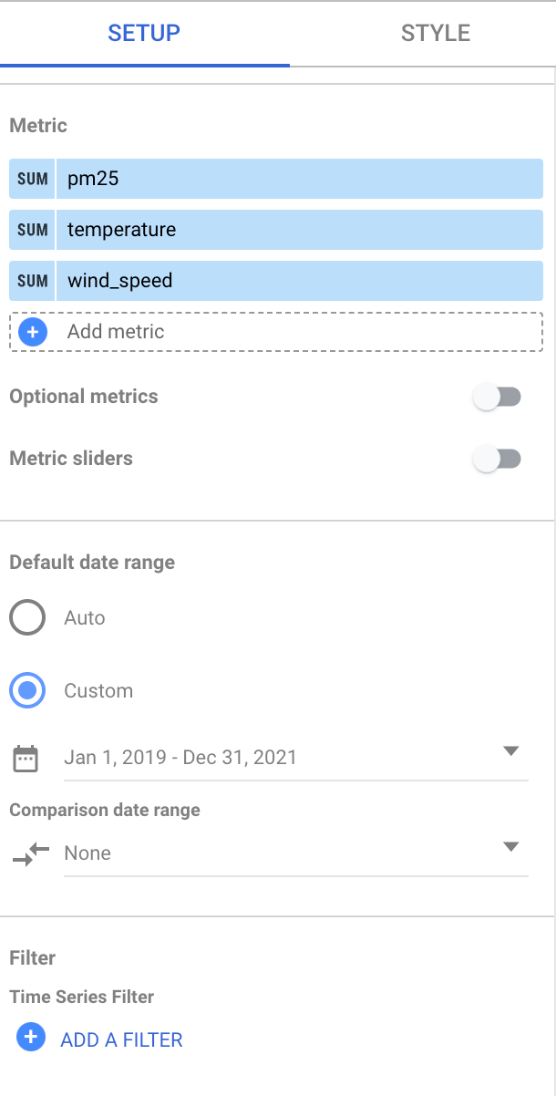
   Looking at the chart, you can see that the input time series has a weekly seasonal pattern.

Note: For more information about Looker Studio support, see Looker Support integrations with Google Cloud.

Create the time series model

Create a time series model to forecast particulate matter values, as represented by the pm25 column, using the pm25, wind_speed, and temperature column values as input variables. Train the model on the air quality data from the bqml_tutorial.seattle_air_quality_daily table, selecting the data gathered between January 1, 2012 and December 31, 2020.

In the following query, the OPTIONS(model_type='ARIMA_PLUS_XREG', time_series_timestamp_col='date', ...) clause indicates that you are creating an ARIMA with external regressors model. The auto_arima option of the CREATE MODEL statement defaults to TRUE, so the auto.ARIMA algorithm automatically tunes the hyperparameters in the model. The algorithm fits dozens of candidate models and chooses the best model, which is the model with the lowest Akaike information criterion (AIC). The data_frequency option of the CREATE MODEL statements defaults to AUTO_FREQUENCY, so the training process automatically infers the data frequency of the input time series. The decompose_time_series option of the CREATE MODEL statement defaults to TRUE, so that information about the time series data is returned when you evaluate the model in the next step.

Follow these steps to create the model:

1. In the Google Cloud console, go to the BigQuery page.

   Go to BigQuery

2. In the query editor, paste in the following query and click Run:

   CREATE OR REPLACE
     MODEL
       `bqml_tutorial.seattle_pm25_xreg_model`
     OPTIONS (
       MODEL_TYPE = 'ARIMA_PLUS_XREG',
       time_series_timestamp_col = 'date',  # Identifies the column that contains time points
       time_series_data_col = 'pm25')       # Identifies the column to forecast
   AS
   SELECT
     date,                                  # The column that contains time points
     pm25,                                  # The column to forecast
     temperature,                           # Temperature input to use in forecasting
     wind_speed                             # Wind speed input to use in forecasting
   FROM
     `bqml_tutorial.seattle_air_quality_daily`
   WHERE
     date
     BETWEEN DATE('2012-01-01')
     AND DATE('2020-12-31');
   

   The query takes about 20 seconds to complete, after which the seattle_pm25_xreg_model model appears in the Explorer pane. Because the query uses a CREATE MODEL statement to create a model, you don't see query results.

Note: You might wonder if United States holidays have an impact on the time series. You can try setting the holiday_region option of the CREATE MODEL statement to US. Setting this option allows a more accurate modeling on holiday time points if there are any holiday patterns in the time series.

Evaluate the candidate models

Evaluate the time series models by using the ML.ARIMA_EVALUATE function. The ML.ARIMA_EVALUATE function shows you the evaluation metrics of all the candidate models that were evaluated during the process of automatic hyperparameter tuning.

Follow these steps to evaluate the model:

1. In the Google Cloud console, go to the BigQuery page.

   Go to BigQuery

2. In the query editor, paste in the following query and click Run:

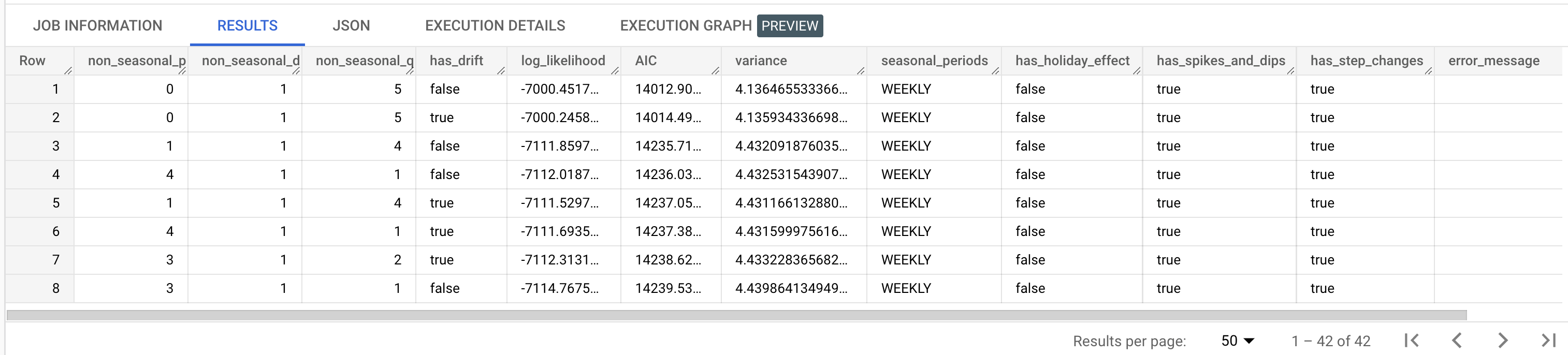
   SELECT
    *
   FROM
    ML.ARIMA_EVALUATE(MODEL `bqml_tutorial.seattle_pm25_xreg_model`);
   

   The results should look similar to the following:

   

   The non_seasonal_p, non_seasonal_d, non_seasonal_q, and has_drift output columns define an ARIMA model in the training pipeline. The log_likelihood, AIC, and varianceoutput columns are relevant to the ARIMA model fitting process.

   The auto.ARIMA algorithm uses the KPSS test to determine the best value for non_seasonal_d, which in this case is 1. When non_seasonal_d is 1, the auto.ARIMA algorithm trains 42 different candidate ARIMA models in parallel. In this example, all 42 candidate models are valid, so the output contains 42 rows, one for each candidate ARIMA model; in cases where some of the models aren't valid, they are excluded from the output. These candidate models are returned in ascending order by AIC. The model in the first row has the lowest AIC, and is considered the best model. The best model is saved as the final model and is used when you call functions such as ML.FORECAST on the model.

   The seasonal_periods column contains information about the seasonal pattern identified in the time series data. It has nothing to do with the ARIMA modeling, therefore it has the same value across all output rows. It reports a weekly pattern, which agrees with the results you saw if you chose to visualize the input data.

   The has_holiday_effect, has_spikes_and_dips, and has_step_changes columns provide information about the input time series data, and are not related to the ARIMA modeling. These columns are returned because the value of the decompose_time_series option in the CREATE MODEL statement is TRUE. These columns also have the same values across all output rows.

   The error_message column shows any errors that incurred during the auto.ARIMA fitting process. One possible reason for errors is when the selected non_seasonal_p, non_seasonal_d, non_seasonal_q, and has_drift columns are not able to stabilize the time series. To retrieve the error message of all the candidate models, set the show_all_candidate_models option to TRUE when you create the model.

   For more information about the output columns, see ML.ARIMA_EVALUATE function.

Inspect the model's coefficients

Inspect the time series model's coefficients by using the ML.ARIMA_COEFFICIENTS function.

Follow these steps to retrieve the model's coefficients:

1. In the Google Cloud console, go to the BigQuery page.

   Go to BigQuery

2. In the query editor, paste in the following query and click Run:

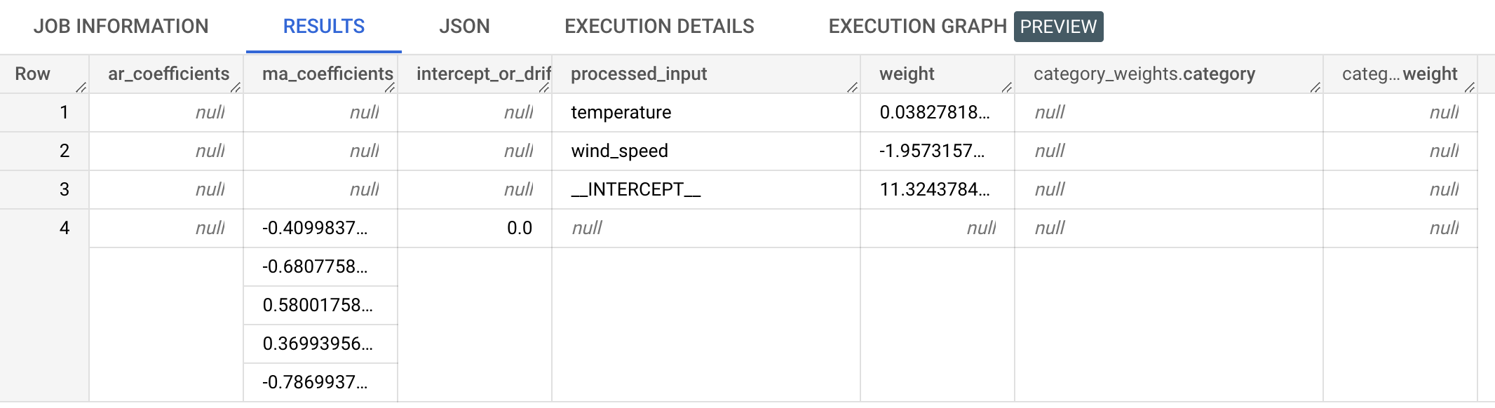
   SELECT
    *
   FROM
    ML.ARIMA_COEFFICIENTS(MODEL `bqml_tutorial.seattle_pm25_xreg_model`);
   

   The results should look similar to the following:

   

   The ar_coefficients output column shows the model coefficients of the autoregressive (AR) part of the ARIMA model. Similarly, the ma_coefficients output column shows the model coefficients of the moving-average (MA) part of the ARIMA model. Both of these columns contain array values, whose lengths are equal to non_seasonal_p and non_seasonal_q, respectively. You saw in the output of the ML.ARIMA_EVALUATE function that the best model has a non_seasonal_p value of 0 and a non_seasonal_q value of 5. Therefore, in the ML.ARIMA_COEFFICIENTS output, the ar_coefficients value is an empty array and the ma_coefficients value is a 5-element array. The intercept_or_drift value is the constant term in the ARIMA model.

   The processed_input, weight, and category_weights output column show the weights for each feature and the intercept in the linear regression model. If the feature is a numerical feature, the weight is in the weight column. If the feature is a categorical feature, the category_weights value is an array of struct values, where each struct value contains the name and weight of a given category.

   For more information about the output columns, see ML.ARIMA_COEFFICIENTS function.

Use the model to forecast data

Forecast future time series values by using the ML.FORECAST function.

In the following GoogleSQL query, the STRUCT(30 AS horizon, 0.8 AS confidence_level) clause indicates that the query forecasts 30 future time points, and generates a prediction interval with a 80% confidence level.

Follow these steps to forecast data with the model:

1. In the Google Cloud console, go to the BigQuery page.

   Go to BigQuery

2. In the query editor, paste in the following query and click Run:

   SELECT
     *
   FROM
     ML.FORECAST(
       MODEL `bqml_tutorial.seattle_pm25_xreg_model`,
       STRUCT(30 AS horizon, 0.8 AS confidence_level),
       (
         SELECT
           date,
           temperature,
           wind_speed
         FROM
           `bqml_tutorial.seattle_air_quality_daily`
         WHERE
           date > DATE('2020-12-31')
       ));
   

   The results should look similar to the following:

   

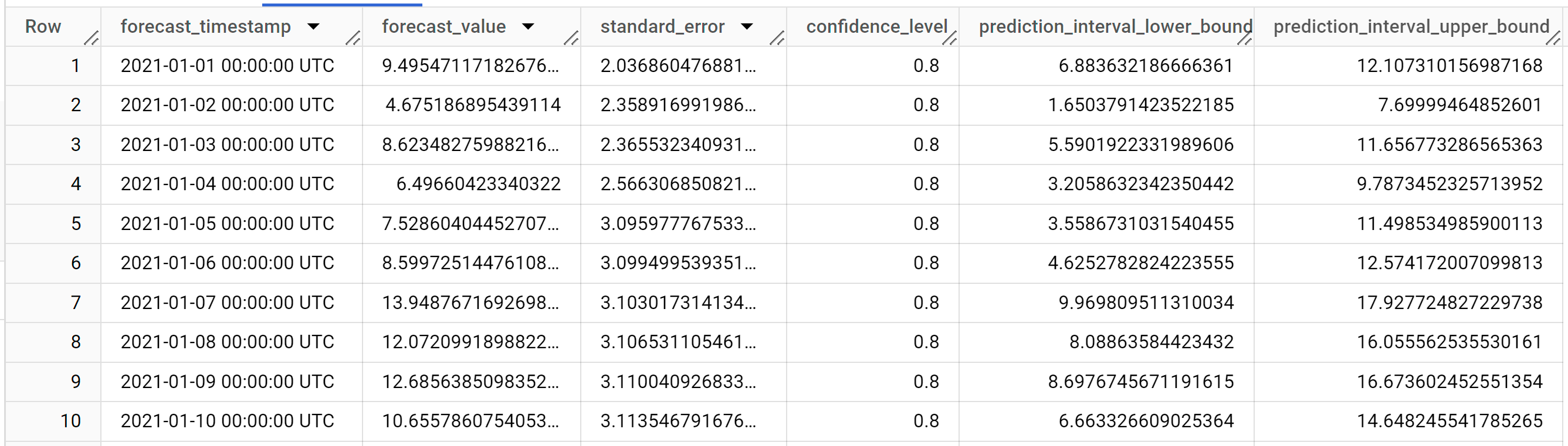
   The output rows are in chronological order by the forecast_timestamp column value. In time series forecasting, the prediction interval, as represented by the prediction_interval_lower_bound and prediction_interval_upper_bound column values, is as important as the forecast_value column value. The forecast_value value is the middle point of the prediction interval. The prediction interval depends on the standard_error and confidence_level column values.

   For more information about the output columns, see ML.FORECAST function.

Evaluate forecasting accuracy

Evaluate the forecasting accuracy of the model by using the ML.EVALUATE function.

In the following GoogleSQL query, the second SELECT statement provides the data with the future features, which are used to forecast the future values to compare to the actual data.

Follow these steps to evaluate the model's accuracy:

1. In the Google Cloud console, go to the BigQuery page.

   Go to BigQuery

2. In the query editor, paste in the following query and click Run:

   SELECT
     *
   FROM
     ML.EVALUATE(
       MODEL `bqml_tutorial.seattle_pm25_xreg_model`,
       (
         SELECT
           date,
           pm25,
           temperature,
           wind_speed
         FROM
           `bqml_tutorial.seattle_air_quality_daily`
         WHERE
           date > DATE('2020-12-31')
       ),
       STRUCT(
         TRUE AS perform_aggregation,
         30 AS horizon));
   

   The results should look similar the following:

   

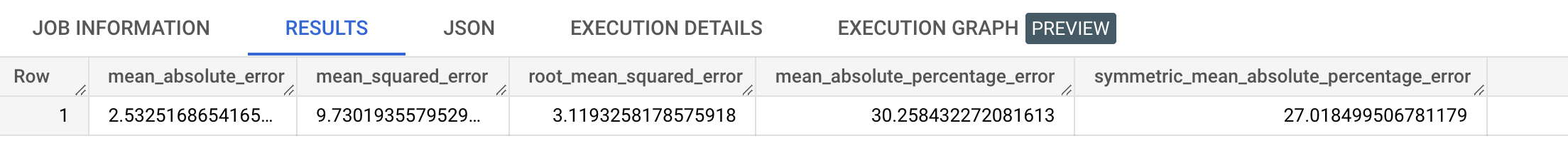
   For more information about the output columns, see ML.EVALUATE function.

Explain the forecasting results

You can get explainability metrics in addition to forecast data by using the ML.EXPLAIN_FORECAST function. The ML.EXPLAIN_FORECAST function forecasts future time series values and also returns all the separate components of the time series.

Similar to the ML.FORECAST function, the STRUCT(30 AS horizon, 0.8 AS confidence_level) clause used in the ML.EXPLAIN_FORECAST function indicates that the query forecasts 30 future time points and generates a prediction interval with 80% confidence.

Follow these steps to explain the model's results:

1. In the Google Cloud console, go to the BigQuery page.

   Go to BigQuery

2. In the query editor, paste in the following query and click Run:

   SELECT
     *
   FROM
     ML.EXPLAIN_FORECAST(
       MODEL `bqml_tutorial.seattle_pm25_xreg_model`,
       STRUCT(30 AS horizon, 0.8 AS confidence_level),
       (
         SELECT
           date,
           temperature,
           wind_speed
         FROM
           `bqml_tutorial.seattle_air_quality_daily`
         WHERE
           date > DATE('2020-12-31')
       ));
   

   The results should look similar to the following:

   

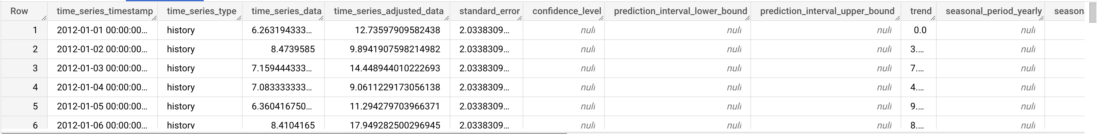
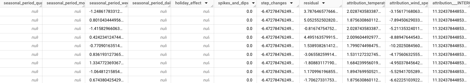
   The output rows are ordered chronologically by the time_series_timestamp column value.

   For more information about the output columns, see ML.EXPLAIN_FORECAST function.

Clean up

To avoid incurring charges to your Google Cloud account for the resources used in this tutorial, either delete the project that contains the resources, or keep the project and delete the individual resources.

• You can delete the project you created.
• Or you can keep the project and delete the dataset.

Delete your dataset

Deleting your project removes all datasets and all tables in the project. If you prefer to reuse the project, you can delete the dataset you created in this tutorial:

1. If necessary, open the BigQuery page in the Google Cloud console.

   Go to the BigQuery page

2. In the navigation, click the bqml_tutorial dataset you created.

3. Click Delete dataset on the right side of the window. This action deletes the dataset, the table, and all the data.

4. In the Delete dataset dialog, confirm the delete command by typing the name of your dataset (bqml_tutorial) and then click Delete.

Delete your project

To delete the project:

Caution: Deleting a project has the following effects:

• Everything in the project is deleted. If you used an existing project for the tasks in this document, when you delete it, you also delete any other work you've done in the project.
• Custom project IDs are lost. When you created this project, you might have created a custom project ID that you want to use in the future. To preserve the URLs that use the project ID, such as an appspot.com URL, delete selected resources inside the project instead of deleting the whole project.

If you plan to explore multiple architectures, tutorials, or quickstarts, reusing projects can help you avoid exceeding project quota limits.

1. In the Google Cloud console, go to the Manage resources page.

   Go to Manage resources

2. In the project list, select the project that you want to delete, and then click Delete.
3. In the dialog, type the project ID, and then click Shut down to delete the project.

What's next

• Learn how to forecast a single time series with a univariate model
• Learn how to forecast multiple time series with a univariate model
• Learn how to scale a univariate model when forecasting multiple time series over many rows.
• Learn how to hierarchically forecast multiple time series with a univariate model
• For an overview of BigQuery ML, see Introduction to AI and ML in BigQuery.