Running TensorFlow inference workloads with TensorRT5 and NVIDIA T4 GPU

---

This tutorial covers how to run deep learning inferences on large scale workloads by using NVIDIA TensorRT5 GPUs running on Compute Engine.

Before you begin, here are some essentials:

• Deep learning inference is the stage in the machine learning process where a trained model is used to recognize, process, and classify results.
• NVIDIA TensorRT is a platform that is optimized for running deep learning workloads.
• GPUs are used to accelerate data-intensive workloads such as machine learning and data processing. A variety of NVIDIA GPUs are available on Compute Engine. This tutorial uses T4 GPUs, since T4 GPUs are specifically designed for deep learning inference workloads.

Objectives

In this tutorial, the following procedures are covered:

• Preparing a model using a pre-trained graph.
• Testing the inference speed for a model with different optimization modes.
• Converting a custom model to TensorRT.
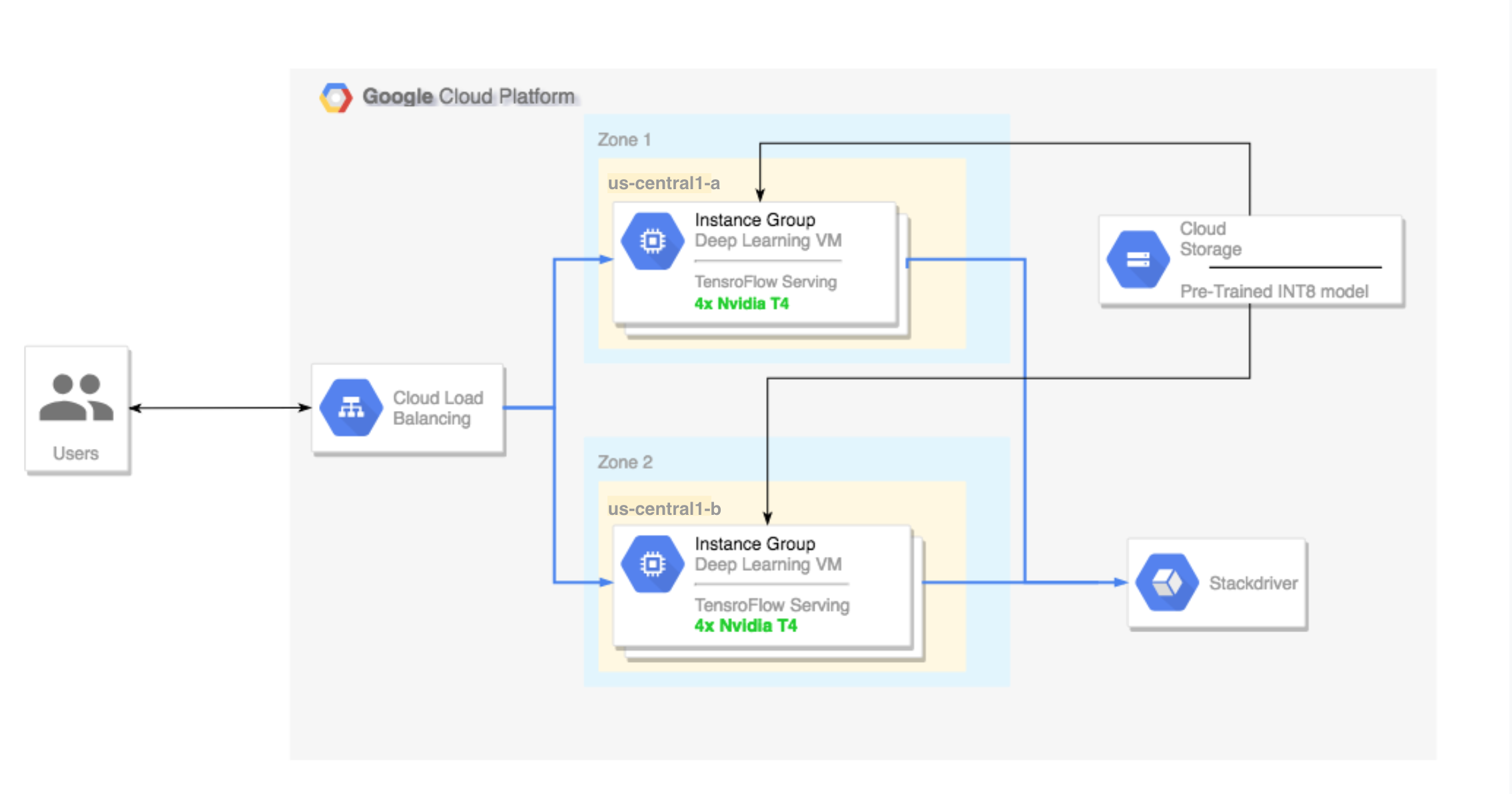
• Setting up a multi-zone cluster. This multi-zone cluster is configured as follows:
  • Built on Deep Learning VM Images. These images are preinstalled with TensorFlow, TensorFlow serving, and TensorRT5.
  • Autoscaling enabled. Autoscaling in this tutorial is based on GPU utilization.
  • Load balancing enabled.
  • Firewall enabled.
• Running an inference workload in the multi-zone cluster.

Costs

The cost of running this tutorial varies by section.

You can calculate the cost by using the pricing calculator.

To estimate the cost to prepare your model and test the inference speeds at different optimization speeds, use the following specifications:

• 1 VM instance: n1-standard-8 (vCPUs: 8, RAM 30GB)
• 1 NVIDIA T4 GPU

To estimate the cost to set up your multi-zone cluster, use the following specifications:

• 2 VM instances: n1-standard-16 (vCPUs: 16, RAM 60GB)
• 4 GPU NVIDIA T4 for each VM instance
• 100 GB SSD for each VM instance
• 1 Forwarding rule

Before you begin

Project setup

1. Sign in to your Google Cloud account. If you're new to Google Cloud, create an account to evaluate how our products perform in real-world scenarios. New customers also get $300 in free credits to run, test, and deploy workloads.

2. In the Google Cloud console, on the project selector page, select or create a Google Cloud project.

   Note: If you don't plan to keep the resources that you create in this procedure, create a project instead of selecting an existing project. After you finish these steps, you can delete the project, removing all resources associated with the project.

   Go to project selector

3. Make sure that billing is enabled for your Google Cloud project.

4. Enable the Compute Engine and Cloud Machine Learning APIs.

   Enable the APIs

5. In the Google Cloud console, on the project selector page, select or create a Google Cloud project.

   Note: If you don't plan to keep the resources that you create in this procedure, create a project instead of selecting an existing project. After you finish these steps, you can delete the project, removing all resources associated with the project.

   Go to project selector

6. Make sure that billing is enabled for your Google Cloud project.

7. Enable the Compute Engine and Cloud Machine Learning APIs.

   Enable the APIs

Tools setup

To use the Google Cloud CLI in this tutorial:

1. Install or update to the latest version of the Google Cloud CLI.
2. (Optional) Set a default region and zone.

Preparing the model

This section covers the creation of a virtual machine (VM) instance that is used to run the model. This section also covers how to download a model from the TensorFlow official models catalog.

1. Create the VM instance. This tutorial is created using the tf-ent-2-10-cu113. For the latest image versions, see Choosing an operating system in the Deep Learning VM Images documentation.

   export IMAGE_FAMILY="tf-ent-2-10-cu113"
   export ZONE="us-central1-b"
   export INSTANCE_NAME="model-prep"
   gcloud compute instances create $INSTANCE_NAME \
      --zone=$ZONE \
      --image-family=$IMAGE_FAMILY \
      --machine-type=n1-standard-8 \
      --image-project=deeplearning-platform-release \
      --maintenance-policy=TERMINATE \
      --accelerator="type=nvidia-tesla-t4,count=1" \
      --metadata="install-nvidia-driver=True"
   

   Note: You can create this instance in any available zone that supports T4 GPUs. A single GPU is enough to compare the different TensorRT optimization modes.

2. Select a model. This tutorial uses the ResNet model. This ResNet model is trained on the ImageNet dataset that is in TensorFlow.

   To download the ResNet model to your VM instance, run the following command:

   wget -q http://download.tensorflow.org/models/official/resnetv2_imagenet_frozen_graph.pb

   Save the location of your ResNet model in the $WORKDIR variable. Replace MODEL_LOCATION with the working directory that contains the downloaded model.

   export WORKDIR=MODEL_LOCATION

Running the inference speed test

This section covers the following procedures:

• Setting up the ResNet model.
• Running inference tests at different optimization modes.
• Reviewing the results of the inference tests.

Overview of the test process

TensorRT can improve the performance speed for inference workloads, however the most significant improvement comes from the quantization process.

Model quantization is the process by which you reduce the precision of weights for a model. For example, if the initial weight of a model is FP32, you can reduce the precision to FP16, INT8, or even INT4. It is important to pick the right compromise between speed (precision of weights) and accuracy of a model. Luckily, TensorFlow includes functionality that does exactly this, measuring accuracy versus speed, or other metrics such as throughput, latency, node conversion rates, and total training time.

Note: This test is limited to image recognition models at the moment, however it should not be too hard to implement a custom test based on this code.

Procedure

1. Set up the ResNet model. To set up the model, run the following commands:

   git clone https://github.com/tensorflow/models.git
   cd models
   git checkout f0e10716160cd048618ccdd4b6e18336223a172f
   touch research/__init__.py
   touch research/tensorrt/__init__.py
   cp research/tensorrt/labellist.json .
   cp research/tensorrt/image.jpg ..
   

2. Run the test. This command takes some time to finish.

   python -m research.tensorrt.tensorrt \
      --frozen_graph=$WORKDIR/resnetv2_imagenet_frozen_graph.pb \
      --image_file=$WORKDIR/image.jpg \
      --native --fp32 --fp16 --int8 \
      --output_dir=$WORKDIR
   

   Where:

   • $WORKDIR is the directory in which you downloaded the ResNet model.
   • The --native arguments are the different quantization modes to test.

3. Review the results. When the test completes, you can do a comparison of the inference results for each optimization mode.

   Predictions:
   Precision:  native [u'seashore, coast, seacoast, sea-coast', u'promontory, headland, head, foreland', u'breakwater, groin, groyne, mole, bulwark, seawall, jetty',     u'lakeside, lakeshore', u'grey whale, gray whale, devilfish, Eschrichtius gibbosus, Eschrichtius robustus']
   Precision:  FP32 [u'seashore, coast, seacoast, sea-coast', u'promontory, headland, head, foreland', u'breakwater, groin, groyne, mole, bulwark, seawall, jetty', u'lakeside,   lakeshore', u'sandbar, sand bar']
   Precision:  FP16 [u'seashore, coast, seacoast, sea-coast', u'promontory, headland, head, foreland', u'breakwater, groin, groyne, mole, bulwark, seawall, jetty', u'lakeside,   lakeshore', u'sandbar, sand bar']
   Precision:  INT8 [u'seashore, coast, seacoast, sea-coast', u'promontory, headland, head, foreland', u'breakwater, groin, groyne, mole, bulwark, seawall, jetty', u'grey         whale, gray whale, devilfish, Eschrichtius gibbosus, Eschrichtius robustus', u'lakeside, lakeshore']
   

   To see the full results, run the following command:

   cat $WORKDIR/log.txt

   

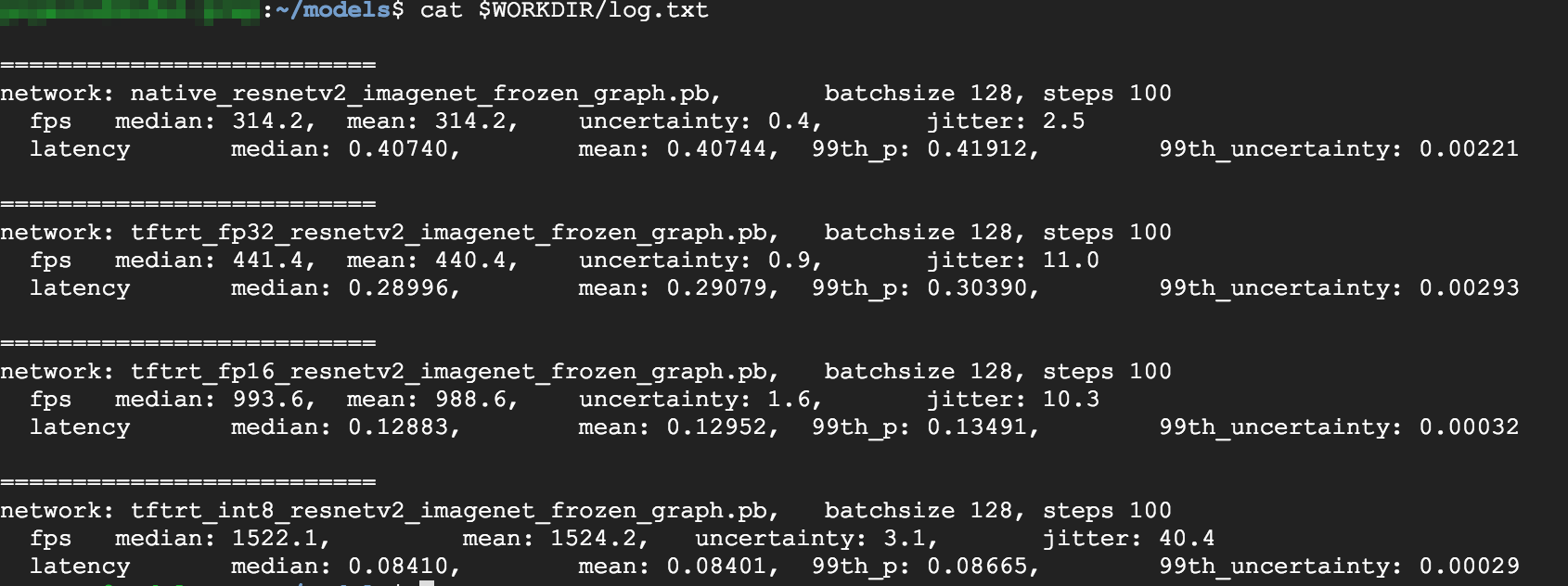
   From the results, you can see that FP32 and FP16 are identical. This means that if you are comfortable working with TensorRT you can definitely start using FP16 right away. INT8, shows slightly worse results.

   In addition, you can see that running the model with TensorRT5 shows the following results:

   • Using FP32 optimization, improves the throughput by 40% from 314 fps to 440 fps. At the same time latency decreases by approximately 30% making it 0.28 ms instead of 0.40 ms.
   • Using FP16 optimization, rather than native TensorFlow graph, increases the speed by 214% from 314 to 988 fps. At the same time latency decreases by 0.12 ms, almost a 3x decrease.
   • Using INT8, you can observe a speedup of 385% from 314 fps to 1524 fps with the latency decreasing to 0.08 ms.

Converting a custom model to TensorRT

For this conversion, you can use an INT8 model.

1. Download the model. To convert a custom model to a TensorRT graph, you need a saved model. To get a saved INT8 ResNet model, run the following command:

   wget http://download.tensorflow.org/models/official/20181001_resnet/savedmodels/resnet_v2_fp32_savedmodel_NCHW.tar.gz
   tar -xzvf resnet_v2_fp32_savedmodel_NCHW.tar.gz

2. Convert the model to the TensorRT graph by using TFTools. To convert the model using the TFTools, run the following command:

   git clone https://github.com/GoogleCloudPlatform/ml-on-gcp.git
   cd ml-on-gcp/dlvm/tools
   python ./convert_to_rt.py \
      --input_model_dir=$WORKDIR/resnet_v2_fp32_savedmodel_NCHW/1538687196 \
      --output_model_dir=$WORKDIR/resnet_v2_int8_NCHW/00001 \
      --batch_size=128 \
      --precision_mode="INT8"
   

   You now have an INT8 model in your $WORKDIR/resnet_v2_int8_NCHW/00001 directory.

   To ensure that everything is set up properly, try to run an inference test.

   tensorflow_model_server --model_base_path=$WORKDIR/resnet_v2_int8_NCHW/ --rest_api_port=8888

3. Upload the model to Cloud Storage. This step is needed so that the model can be used from the multiple-zone cluster that is set up in the next section. To upload the model, complete the following steps:

   1. Archive the model.

      tar -zcvf model.tar.gz ./resnet_v2_int8_NCHW/

   2. Upload the archive. Replace GCS_PATH with the path to your Cloud Storage bucket.

      export GCS_PATH=GCS_PATH
      gcloud storage cp model.tar.gz $GCS_PATH
      

      If needed, you can get an INT8 frozen graph from the Cloud Storage at this URL:

      gs://cloud-samples-data/dlvm/t4/model.tar.gz

Setting up a multiple-zone cluster

Create the cluster

Now that you have a model on the Cloud Storage platform, you can create a cluster.

1. Create an instance template. An instance template is a useful resource to creates new instances. See Instance Templates. Replace YOUR_PROJECT_NAME with your project ID.

   export INSTANCE_TEMPLATE_NAME="tf-inference-template"
   export IMAGE_FAMILY="tf-ent-2-10-cu113"
   export PROJECT_NAME=YOUR_PROJECT_NAME
   
   gcloud beta compute --project=$PROJECT_NAME instance-templates create $INSTANCE_TEMPLATE_NAME \
        --machine-type=n1-standard-16 \
        --maintenance-policy=TERMINATE \
        --accelerator=type=nvidia-tesla-t4,count=4 \
        --min-cpu-platform=Intel\ Skylake \
        --tags=http-server,https-server \
        --image-family=$IMAGE_FAMILY \
        --image-project=deeplearning-platform-release \
        --boot-disk-size=100GB \
        --boot-disk-type=pd-ssd \
        --boot-disk-device-name=$INSTANCE_TEMPLATE_NAME \
        --metadata startup-script-url=gs://cloud-samples-data/dlvm/t4/start_agent_and_inf_server_4.sh
   

   • This instance template includes a startup script that is specified by the metadata parameter.
     • Run this startup script during instance creation on every instance that uses this template.
     • This startup script performs the following steps:
       • Installs a monitoring agent that monitors the GPU usage on the instance.
       • Downloads the model.
       • Starts the inference service.
     • In the startup script, tf_serve.py contains the inference logic. This example includes a very small python file based on the TFServe package.
     • To view the startup script, see startup_inf_script.sh.

2. Create a managed instance group (MIG). This managed instance group is needed to set up multiple running instances in specific zones. The instances are created based on the instance template generated in the previous step.

   export INSTANCE_GROUP_NAME="deeplearning-instance-group"
   export INSTANCE_TEMPLATE_NAME="tf-inference-template"
   gcloud compute instance-groups managed create $INSTANCE_GROUP_NAME \
      --template $INSTANCE_TEMPLATE_NAME \
      --base-instance-name deeplearning-instances \
      --size 2 \
      --zones us-central1-a,us-central1-b
   

   Note: INSTANCE_TEMPLATE_NAME is the name of the instance template that you created in the previous step.
   • You can create this instance in any available zone that support T4 GPUs. Ensure that you have available GPU quotas in the zone.

   • The creation of the instance takes some time. You can watch the progress by running the following commands:

     export INSTANCE_GROUP_NAME="deeplearning-instance-group"

     gcloud compute instance-groups managed list-instances $INSTANCE_GROUP_NAME --region us-central1

     

   • When the managed instance group is created, you should see an output that resembles the following:

     

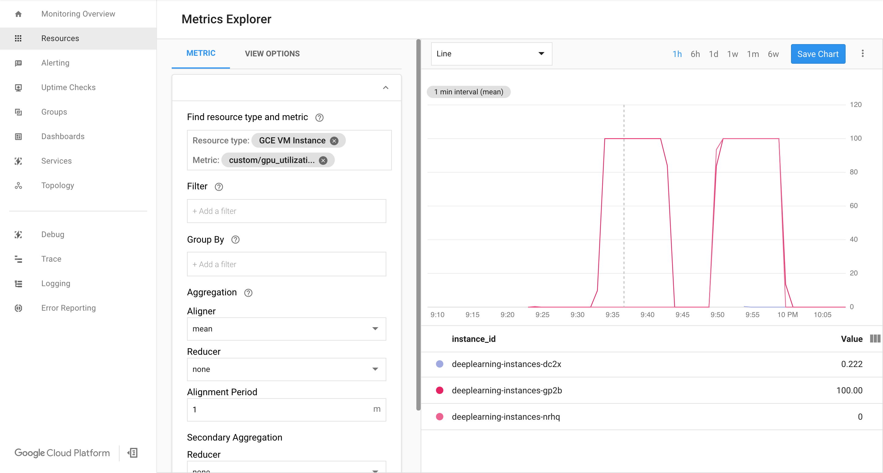
3. Confirm that metrics are available on the Google Cloud Cloud Monitoring page.

   1. In the Google Cloud console, go to the Monitoring page.

      Go to Monitoring

   2. If Metrics Explorer is shown in the navigation pane, click Metrics Explorer. Otherwise, select Resources and then select Metrics Explorer.

   3. Search for gpu_utilization.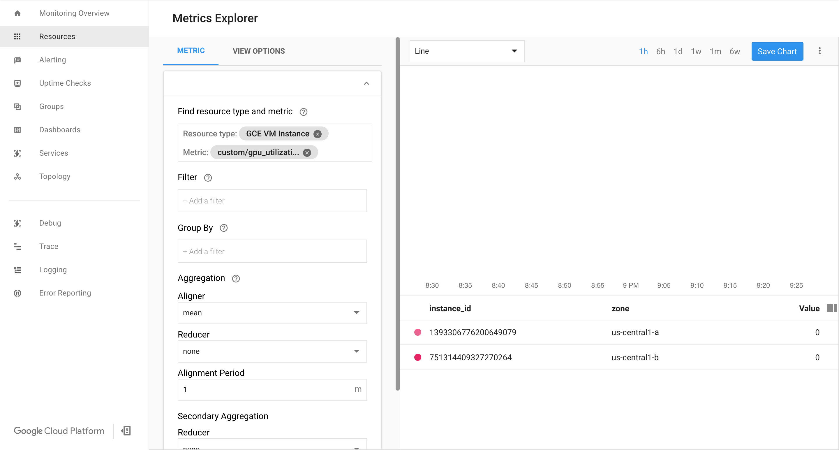

      

   4. If data is coming in, you should see something like this:

      

Enable autoscaling

1. Enable autoscaling for the managed instance group.

   export INSTANCE_GROUP_NAME="deeplearning-instance-group"
   
   gcloud compute instance-groups managed set-autoscaling $INSTANCE_GROUP_NAME \
      --custom-metric-utilization metric=custom.googleapis.com/gpu_utilization,utilization-target-type=GAUGE,utilization-target=85 \
      --max-num-replicas 4 \
      --cool-down-period 360 \
      --region us-central1
   

   The custom.googleapis.com/gpu_utilization is the full path to our metric. The sample specifies level 85, this means that whenever GPU utilization reaches 85, the platform creates a new instance in our group.

2. Test the autoscaling. To test the autoscaling, you need to perform the following steps:

   1. SSH to the instance. See Connecting to Instances.

   2. Use the gpu-burn tool to load your GPU to 100% utilization for 600 seconds:

      git clone https://github.com/GoogleCloudPlatform/ml-on-gcp.git
      cd ml-on-gcp/third_party/gpu-burn
      git checkout c0b072aa09c360c17a065368294159a6cef59ddf
      make
      ./gpu_burn 600 > /dev/null &
      

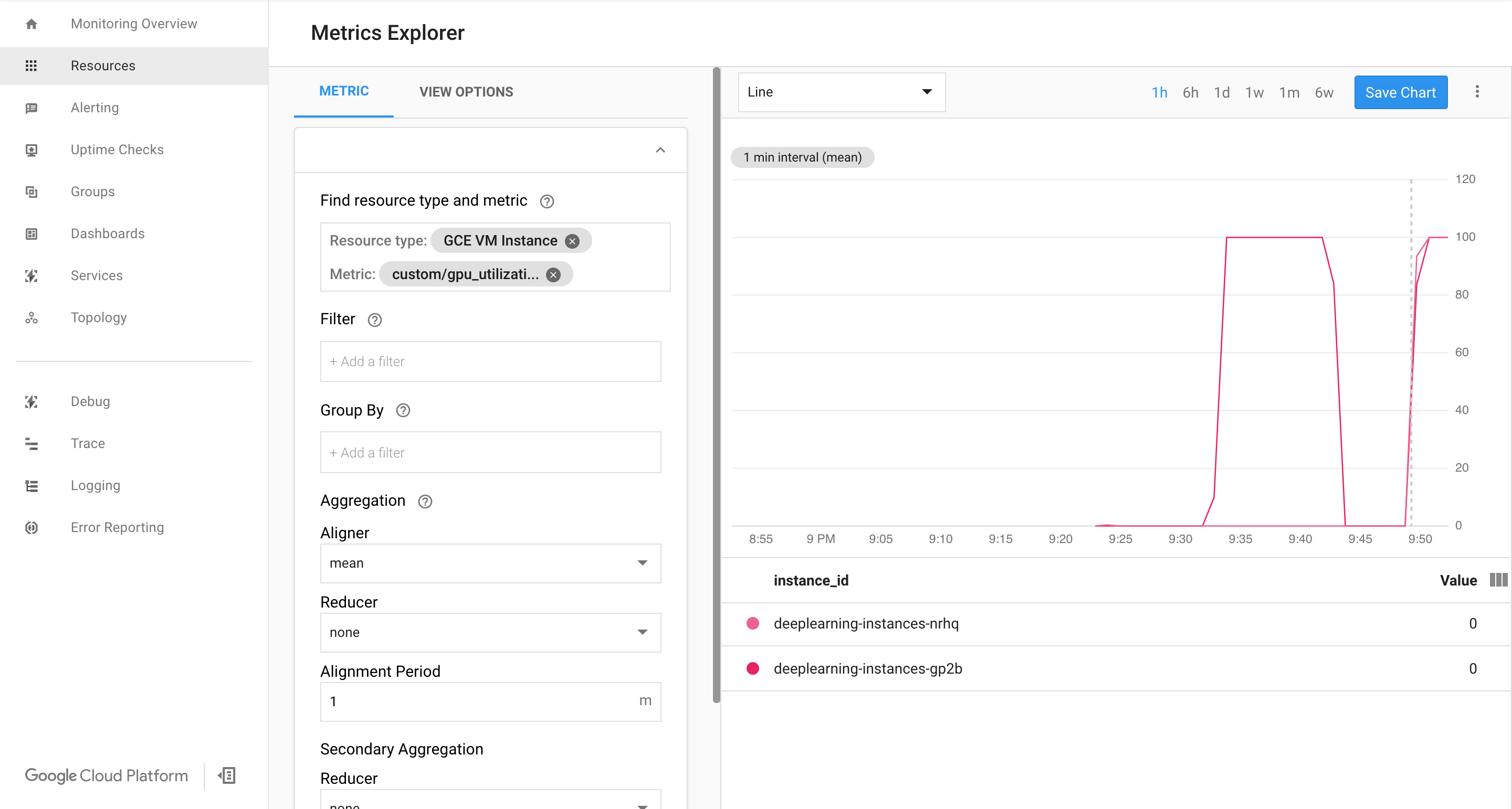
   3. View the Cloud Monitoring page. Observe the autoscaling. The cluster scales up by adding one more instance.

      

   4. In the Google Cloud console, go to the Instance groups page.

      Go to Instance groups

   5. Click the deeplearning-instance-group managed instance group.

   6. Click the Monitoring tab.

      At this point your autoscaling logic should be trying to spin as much instances as possible to reduce the load, without any luck:

      

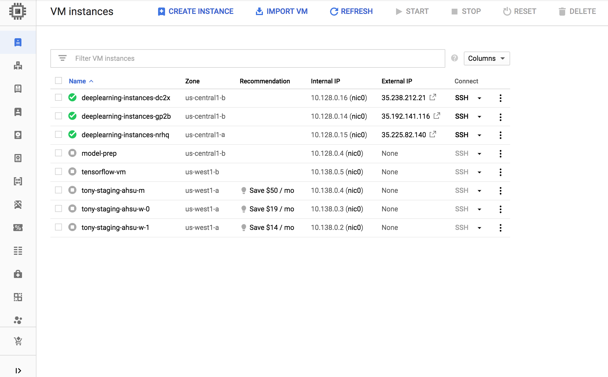
      At this point you can stop burning instances, and observe how the system scales down.

Set up a load balancer

Let's revisit what you have so far:

• A trained model, optimized with TensorRT5 (INT8)
• A managed group of instances. These instances have auto scaling enable based on the GPU utilization enabled

Now you can create a load balancer in front of the instances.

1. Create health checks. Health checks are used to determine if a particular host on our backend can serve the traffic.

   export HEALTH_CHECK_NAME="http-basic-check"
   
   gcloud compute health-checks create http $HEALTH_CHECK_NAME \
      --request-path /v1/models/default \
      --port 8888
   

2. Create a backend service that includes an instance group and health check.

   1. Create the health check.

      export HEALTH_CHECK_NAME="http-basic-check"
      export WEB_BACKED_SERVICE_NAME="tensorflow-backend"
      
      gcloud compute backend-services create $WEB_BACKED_SERVICE_NAME \
         --protocol HTTP \
         --health-checks $HEALTH_CHECK_NAME \
         --global
      

   2. Add the instance group to the new backend service.

      export INSTANCE_GROUP_NAME="deeplearning-instance-group"
      export WEB_BACKED_SERVICE_NAME="tensorflow-backend"
      
      gcloud compute backend-services add-backend $WEB_BACKED_SERVICE_NAME \
         --balancing-mode UTILIZATION \
         --max-utilization 0.8 \
         --capacity-scaler 1 \
         --instance-group $INSTANCE_GROUP_NAME \
         --instance-group-region us-central1 \
         --global
      

3. Set up forwarding URL. The load balancer needs to know which URL can be forwarded to the backends services.

   export WEB_BACKED_SERVICE_NAME="tensorflow-backend"
   export WEB_MAP_NAME="map-all"
   
   gcloud compute url-maps create $WEB_MAP_NAME \
      --default-service $WEB_BACKED_SERVICE_NAME
   

4. Create the load balancer.

   export WEB_MAP_NAME="map-all"
   export LB_NAME="tf-lb"
   
   gcloud compute target-http-proxies create $LB_NAME \
      --url-map $WEB_MAP_NAME
   

5. Add an external IP address to the load balancer.

   export IP4_NAME="lb-ip4"
   
   gcloud compute addresses create $IP4_NAME \
      --ip-version=IPV4 \
      --network-tier=PREMIUM \
      --global
   

6. Find the IP address that is allocated.

   gcloud compute addresses list

7. Set up the forwarding rule that tells Google Cloud to forward all requests from the public IP address to the load balancer.

   export IP=$(gcloud compute addresses list | grep ${IP4_NAME} | awk '{print $2}')
   export LB_NAME="tf-lb"
   export FORWARDING_RULE="lb-fwd-rule"
   
   gcloud compute forwarding-rules create $FORWARDING_RULE \
      --address $IP \
      --global \
      --load-balancing-scheme=EXTERNAL \
      --network-tier=PREMIUM \
      --target-http-proxy $LB_NAME \
      --ports 80
   

   After creating the global forwarding rules, it can take several minutes for your configuration to propagate.

Enable firewall

1. Check if you have firewall rules that allow connections from external sources to your VM instances.

   gcloud compute firewall-rules list

2. If you do not have firewall rules to allow these connections, you must create them. To create firewall rules, run the following commands:

   gcloud compute firewall-rules create www-firewall-80 \
      --target-tags http-server --allow tcp:80
   
   gcloud compute firewall-rules create www-firewall-8888 \
      --target-tags http-server --allow tcp:8888
   

Running an inference

1. You can use the following python script to convert images to a format that can uploaded to the server.

   from PIL import Image
   import numpy as np
   import json
   import codecs
   
   
   img = Image.open("image.jpg").resize((240, 240))
   img_array=np.array(img)
   result = {
         "instances":[img_array.tolist()]
          }
   file_path="/tmp/out.json"
   print(json.dump(result, codecs.open(file_path, 'w', encoding='utf-8'), separators=(',', ':'), sort_keys=True, indent=4))
   

2. Run the inference.

   curl -X POST $IP/v1/models/default:predict -d @/tmp/out.json

Clean up

To avoid incurring charges to your Google Cloud account for the resources used in this tutorial, either delete the project that contains the resources, or keep the project and delete the individual resources.

1. Delete forwarding rules.

   gcloud compute forwarding-rules delete $FORWARDING_RULE --global

2. Delete the IPV4 address.

   gcloud compute addresses delete $IP4_NAME --global

3. Delete the load balancer.

   gcloud compute target-http-proxies delete $LB_NAME

4. Delete the forwarding URL.

   gcloud compute url-maps delete $WEB_MAP_NAME

5. Delete the backend service.

   gcloud compute backend-services delete $WEB_BACKED_SERVICE_NAME --global

6. Delete health checks.

   gcloud compute health-checks delete $HEALTH_CHECK_NAME

7. Delete the managed instance group.

   gcloud compute instance-groups managed delete $INSTANCE_GROUP_NAME --region us-central1

8. Delete the instance template.

   gcloud beta compute --project=$PROJECT_NAME instance-templates delete $INSTANCE_TEMPLATE_NAME

9. Delete the firewall rules.

   gcloud compute firewall-rules delete www-firewall-80

   gcloud compute firewall-rules delete www-firewall-8888