Build and use a classification model on census data

---

In this tutorial, you use a binary logistic regression model in BigQuery ML to predict the income range of individuals based on their demographic data. A binary logistic regression model predicts whether a value falls into one of two categories, in this case whether an individual's annual income falls above or below $50,000.

This tutorial uses the bigquery-public-data.ml_datasets.census_adult_income dataset. This dataset contains the demographic and income information of US residents from 2000 and 2010.

Objectives

In this tutorial you will perform the following tasks:

• Create a logistic regression model.
• Evaluate the model.
• Make predictions by using the model.
• Explain the results produced by the model.

Costs

This tutorial uses billable components of Google Cloud, including the following:

• BigQuery
• BigQuery ML

For more information on BigQuery costs, see the BigQuery pricing page.

For more information on BigQuery ML costs, see BigQuery ML pricing.

Before you begin

1. In the Google Cloud console, on the project selector page, select or create a Google Cloud project.

   Note: If you don't plan to keep the resources that you create in this procedure, create a project instead of selecting an existing project. After you finish these steps, you can delete the project, removing all resources associated with the project.

   Go to project selector

2. Verify that billing is enabled for your Google Cloud project.

3. Enable the BigQuery API.

   Enable the API

Required permissions

To create the model using BigQuery ML, you need the following IAM permissions:

• bigquery.jobs.create
• bigquery.models.create
• bigquery.models.getData
• bigquery.models.updateData
• bigquery.models.updateMetadata

To run inference, you need the following permissions:

• bigquery.models.getData on the model
• bigquery.jobs.create

Introduction

A common task in machine learning is to classify data into one of two types, known as labels. For example, a retailer might want to predict whether a given customer will purchase a new product, based on other information about that customer. In that case, the two labels might be will buy and won't buy. The retailer can construct a dataset such that one column represents both labels, and also contains customer information such as the customer's location, their previous purchases, and their reported preferences. The retailer can then use a binary logistic regression model that uses this customer information to predict which label best represents each customer.

In this tutorial, you create a binary logistic regression model that predicts whether a US Census respondent's income falls into one of two ranges based on the respondent's demographic attributes.

Create a dataset

Create a BigQuery dataset to store your model:

1. In the Google Cloud console, go to the BigQuery page.

   Go to BigQuery

2. In the Explorer pane, click your project name.

3. Click View actions > Create dataset.

4. On the Create dataset page, do the following:

   • For Dataset ID, enter census.

   • For Location type, select Multi-region, and then select US (multiple regions in United States).

     The public datasets are stored in the US multi-region. For simplicity, store your dataset in the same location.

   • Leave the remaining default settings as they are, and click Create dataset.

Examine the data

Examine the dataset and identify which columns to use as training data for the logistic regression model. Select 100 rows from the census_adult_income table:

SQL

1. In the Google Cloud console, go to the BigQuery page.

   Go to BigQuery

2. In the query editor, run the following GoogleSQL query:

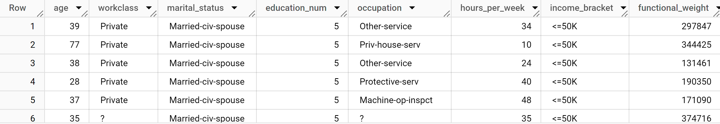
   SELECT
   age,
   workclass,
   marital_status,
   education_num,
   occupation,
   hours_per_week,
   income_bracket,
   functional_weight
   FROM
   `bigquery-public-data.ml_datasets.census_adult_income`
   LIMIT
   100;

3. The results look similar to the following:

   

BigQuery DataFrames

Before trying this sample, follow the BigQuery DataFrames setup instructions in the BigQuery quickstart using BigQuery DataFrames. For more information, see the BigQuery DataFrames reference documentation.

To authenticate to BigQuery, set up Application Default Credentials. For more information, see Set up ADC for a local development environment.

import bigframes.pandas as bpd

df = bpd.read_gbq(
    "bigquery-public-data.ml_datasets.census_adult_income",
    columns=(
        "age",
        "workclass",
        "marital_status",
        "education_num",
        "occupation",
        "hours_per_week",
        "income_bracket",
        "functional_weight",
    ),
    max_results=100,
)
df.peek()
# Output:
# age      workclass       marital_status  education_num          occupation  hours_per_week income_bracket  functional_weight
#  47      Local-gov   Married-civ-spouse             13      Prof-specialty              40           >50K             198660
#  56        Private        Never-married              9        Adm-clerical              40          <=50K              85018
#  40        Private   Married-civ-spouse             12        Tech-support              40           >50K             285787
#  34   Self-emp-inc   Married-civ-spouse              9        Craft-repair              54           >50K             207668
#  23        Private   Married-civ-spouse             10   Handlers-cleaners              40          <=50K              40060

The query results show that the income_bracket column in the census_adult_income table has only one of two values: <=50K or >50K.

Prepare the sample data

In this tutorial, you predict census respondent income based on values of the following columns in the census_adult_income table:

• age: the age of the respondent.
• workclass: class of work performed. For example local government, private, or self-employed.
• marital_status
• education_num: the respondent's higheset level of education.
• occupation
• hours_per_week: hours worked per week.

You exclude columns that duplicate data. For example, the education column, because the education and education_num column values express the same data in different formats.

The functional_weight column is the number of individuals that the census organization believes a particular row represents. Because the value of this column is unrelated to the value of the income_bracket for any given row, you use the value in this column to separate the data into training, evaluation, and prediction sets by creating a new dataframe column that is derived from the functional_weight column. You label 80% of the data for training the model, 10% of data for evaluation, and 10% of the data for prediction.

SQL

Create a view a view with the sample data. This view is used by the CREATE MODEL statement later in this tutorial.

Run the query that prepares the sample data:

1. In the Google Cloud console, go to the BigQuery page.

   Go to BigQuery

2. In the query editor, run the following query:

   CREATE OR REPLACE VIEW
   `census.input_data` AS
   SELECT
   age,
   workclass,
   marital_status,
   education_num,
   occupation,
   hours_per_week,
   income_bracket,
   CASE
     WHEN MOD(functional_weight, 10) < 8 THEN 'training'
     WHEN MOD(functional_weight, 10) = 8 THEN 'evaluation'
     WHEN MOD(functional_weight, 10) = 9 THEN 'prediction'
   END AS dataframe
   FROM
   `bigquery-public-data.ml_datasets.census_adult_income`;

3. View the sample data:

   SELECT * FROM `census.input_data`;

BigQuery DataFrames

Create a DataFrame called input_data. You use input_data later in this tutorial to use to train the model, evaluate it, and make predictions.

Before trying this sample, follow the BigQuery DataFrames setup instructions in the BigQuery quickstart using BigQuery DataFrames. For more information, see the BigQuery DataFrames reference documentation.

To authenticate to BigQuery, set up Application Default Credentials. For more information, see Set up ADC for a local development environment.

import bigframes.pandas as bpd

input_data = bpd.read_gbq(
    "bigquery-public-data.ml_datasets.census_adult_income",
    columns=(
        "age",
        "workclass",
        "marital_status",
        "education_num",
        "occupation",
        "hours_per_week",
        "income_bracket",
        "functional_weight",
    ),
)
input_data["dataframe"] = bpd.Series("training", index=input_data.index,).case_when(
    [
        (((input_data["functional_weight"] % 10) == 8), "evaluation"),
        (((input_data["functional_weight"] % 10) == 9), "prediction"),
    ]
)
del input_data["functional_weight"]

Create a logistic regression model

Create a logistic regression model with the training data you labeled in the previous section.

SQL

Use the CREATE MODEL statement and specify LOGISTIC_REG for the model type.

The following are useful things to know about the CREATE MODEL statement:

• The input_label_cols option specifies which column in the SELECT statement to use as the label column. Here, the label column is income_bracket, so the model learns which of the two values of income_bracket is most likely for a given row based on the other values present in that row.

• It is not necessary to specify whether a logistic regression model is binary or multiclass. BigQuery ML determines which type of model to train based on the number of unique values in the label column.

• The auto_class_weights option is set to TRUE in order to balance the class labels in the training data. By default, the training data is unweighted. If the labels in the training data are imbalanced, the model may learn to predict the most popular class of labels more heavily. In this case, most of the respondents in the dataset are in the lower income bracket. This may lead to a model that predicts the lower income bracket too heavily. Class weights balance the class labels by calculating the weights for each class in inverse proportion to the frequency of that class.

• The enable_global_explain option is set to TRUE in order to let you use the ML.GLOBAL_EXPLAIN function on the model later in the tutorial.

• The SELECT statement queries the input_data view that contains the sample data. The WHERE clause filters the rows so that only those rows labeled as training data are used to train the model.

Run the query that creates your logistic regression model:

1. In the Google Cloud console, go to the BigQuery page.

   Go to BigQuery

2. In the query editor, run the following query:

   CREATE OR REPLACE MODEL
   `census.census_model`
   OPTIONS
   ( model_type='LOGISTIC_REG',
     auto_class_weights=TRUE,
     enable_global_explain=TRUE,
     data_split_method='NO_SPLIT',
     input_label_cols=['income_bracket'],
     max_iterations=15) AS
   SELECT * EXCEPT(dataframe)
   FROM
   `census.input_data`
   WHERE
   dataframe = 'training'

3. In the Explorer pane, click Datasets.

4. In the Datasets pane, click census.

5. Click the Models pane.

6. Click census_model.

7. The Details tab lists the attributes that BigQuery ML used to perform logistic regression.

BigQuery DataFrames

Use the fit method to train the model and the to_gbq method to save it to your dataset.

Before trying this sample, follow the BigQuery DataFrames setup instructions in the BigQuery quickstart using BigQuery DataFrames. For more information, see the BigQuery DataFrames reference documentation.

To authenticate to BigQuery, set up Application Default Credentials. For more information, see Set up ADC for a local development environment.

import bigframes.ml.linear_model

# input_data is defined in an earlier step.
training_data = input_data[input_data["dataframe"] == "training"]
X = training_data.drop(columns=["income_bracket", "dataframe"])
y = training_data["income_bracket"]

census_model = bigframes.ml.linear_model.LogisticRegression(
    # Balance the class labels in the training data by setting
    # class_weight="balanced".
    #
    # By default, the training data is unweighted. If the labels
    # in the training data are imbalanced, the model may learn to
    # predict the most popular class of labels more heavily. In
    # this case, most of the respondents in the dataset are in the
    # lower income bracket. This may lead to a model that predicts
    # the lower income bracket too heavily. Class weights balance
    # the class labels by calculating the weights for each class in
    # inverse proportion to the frequency of that class.
    class_weight="balanced",
    max_iterations=15,
)
census_model.fit(X, y)

census_model.to_gbq(
    your_model_id,  # For example: "your-project.census.census_model"
    replace=True,
)

Evaluate the model's performance

After creating the model, evaluate the model's performance against the evaluation data.

SQL

The ML.EVALUATE function function evaluates the predicted values generated by the model against the evaluation data.

For input, the ML.EVALUATE function takes the trained model and the rows from theinput_data view that have evaluation as the dataframe column value. The function returns a single row of statistics about the model.

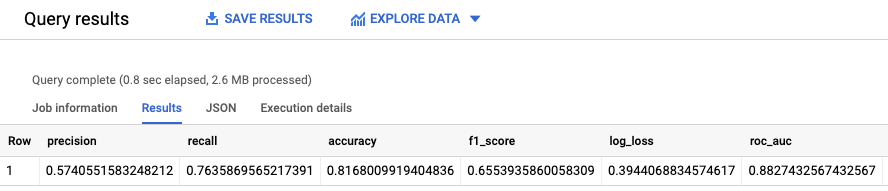
Run the ML.EVALUATE query:

1. In the Google Cloud console, go to the BigQuery page.

   Go to BigQuery

2. In the query editor, run the following query:

   SELECT
   *
   FROM
   ML.EVALUATE (MODEL `census.census_model`,
     (
     SELECT
       *
     FROM
       `census.input_data`
     WHERE
       dataframe = 'evaluation'
     )
   );

3. The results look similar to the following:

   

BigQuery DataFrames

Use the score method to evaluate model against the actual data.

Before trying this sample, follow the BigQuery DataFrames setup instructions in the BigQuery quickstart using BigQuery DataFrames. For more information, see the BigQuery DataFrames reference documentation.

To authenticate to BigQuery, set up Application Default Credentials. For more information, see Set up ADC for a local development environment.

# Select model you'll use for predictions. `read_gbq_model` loads model
# data from BigQuery, but you could also use the `census_model` object
# from previous steps.
census_model = bpd.read_gbq_model(
    your_model_id,  # For example: "your-project.census.census_model"
)

# input_data is defined in an earlier step.
evaluation_data = input_data[input_data["dataframe"] == "evaluation"]
X = evaluation_data.drop(columns=["income_bracket", "dataframe"])
y = evaluation_data["income_bracket"]

# The score() method evaluates how the model performs compared to the
# actual data. Output DataFrame matches that of ML.EVALUATE().
score = census_model.score(X, y)
score.peek()
# Output:
#    precision    recall  accuracy  f1_score  log_loss   roc_auc
# 0   0.685764  0.536685   0.83819  0.602134  0.350417  0.882953

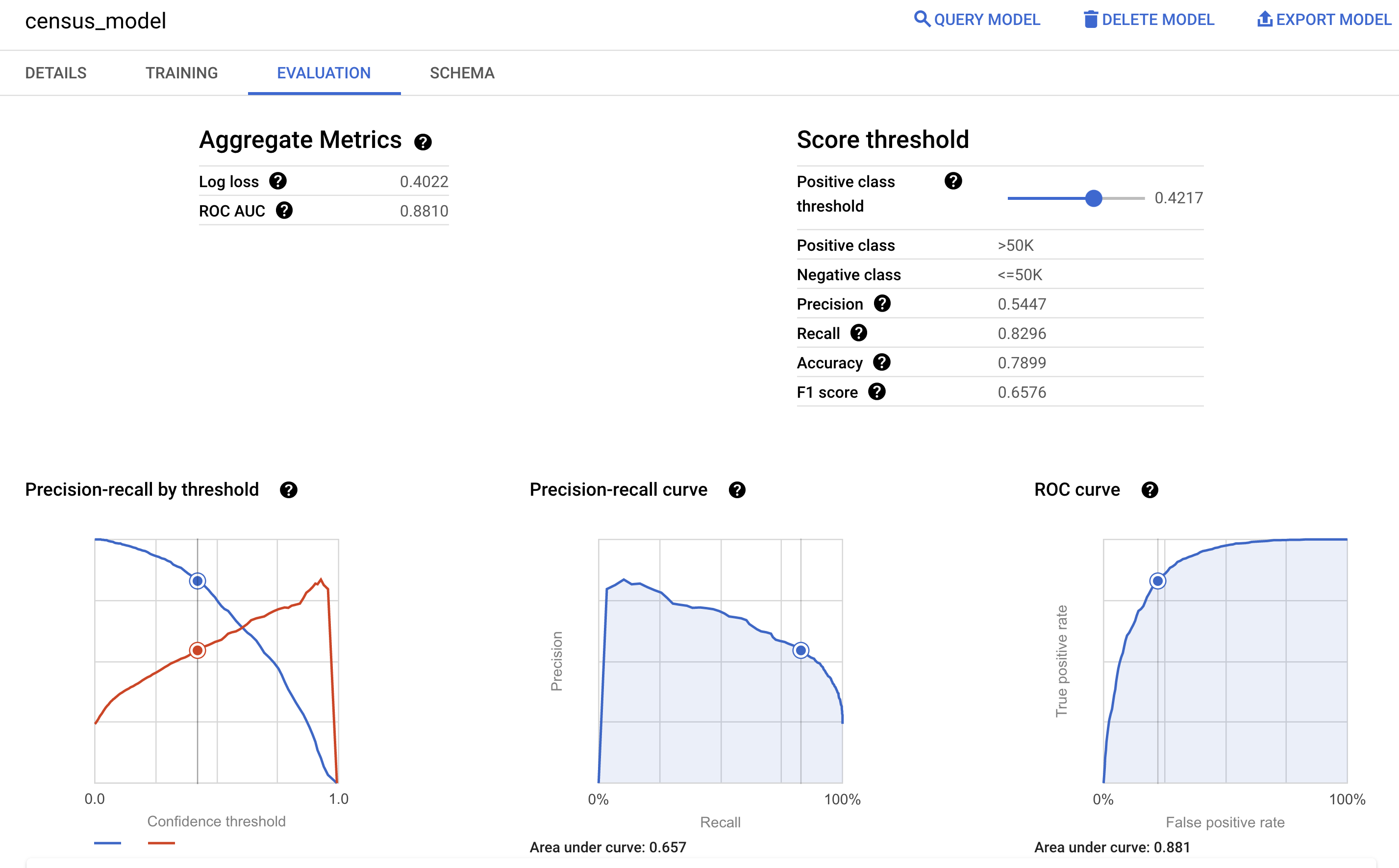
You can also look at the model's Evaluation pane in the Google Cloud console to view the evaluation metrics calculated during the training:

Predict the income bracket

Use the model to predict the most likely income bracket for each respondent.

SQL

Use the ML.PREDICT function to make predictions about the likely income bracket. For input, the ML.PREDICT function takes the trained model and the rows from the input_data view that have prediction as the dataframe column value.

Run the ML.PREDICT query:

1. In the Google Cloud console, go to the BigQuery page.

   Go to BigQuery

2. In the query editor, run the following query:

   SELECT
   *
   FROM
   ML.PREDICT (MODEL `census.census_model`,
     (
     SELECT
       *
     FROM
       `census.input_data`
     WHERE
       dataframe = 'prediction'
     )
   );

3. The results look similar to the following:

   

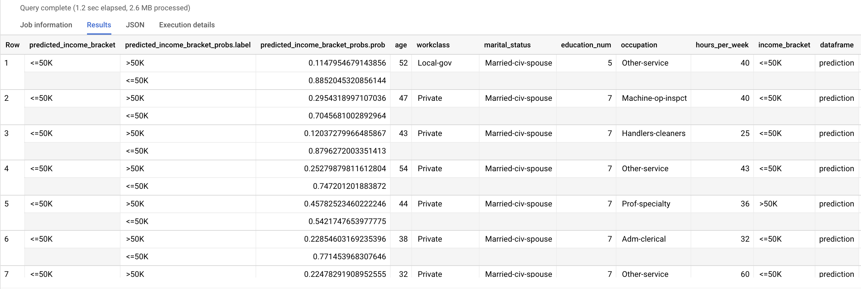
The predicted_income_bracket column contains the predicted income bracket for the respondent.

BigQuery DataFrames

Use the predict method to make predictions about the likely income bracket.

Before trying this sample, follow the BigQuery DataFrames setup instructions in the BigQuery quickstart using BigQuery DataFrames. For more information, see the BigQuery DataFrames reference documentation.

To authenticate to BigQuery, set up Application Default Credentials. For more information, see Set up ADC for a local development environment.

# Select model you'll use for predictions. `read_gbq_model` loads model
# data from BigQuery, but you could also use the `census_model` object
# from previous steps.
census_model = bpd.read_gbq_model(
    your_model_id,  # For example: "your-project.census.census_model"
)

# input_data is defined in an earlier step.
prediction_data = input_data[input_data["dataframe"] == "prediction"]

predictions = census_model.predict(prediction_data)
predictions.peek()
# Output:
#           predicted_income_bracket                     predicted_income_bracket_probs  age workclass  ... occupation  hours_per_week income_bracket   dataframe
# 18004                    <=50K  [{'label': ' >50K', 'prob': 0.0763305999358786...   75         ?  ...          ?               6          <=50K  prediction
# 18886                    <=50K  [{'label': ' >50K', 'prob': 0.0448866871906495...   73         ?  ...          ?              22           >50K  prediction
# 31024                    <=50K  [{'label': ' >50K', 'prob': 0.0362982319421936...   69         ?  ...          ?               1          <=50K  prediction
# 31022                    <=50K  [{'label': ' >50K', 'prob': 0.0787836112058324...   75         ?  ...          ?               5          <=50K  prediction
# 23295                    <=50K  [{'label': ' >50K', 'prob': 0.3385373037905673...   78         ?  ...          ?              32          <=50K  prediction

Explain the prediction results

To understand why the model is generating these prediction results, you can use the ML.EXPLAIN_PREDICT function.

ML.EXPLAIN_PREDICT is an extended version of the ML.PREDICT function. ML.EXPLAIN_PREDICT not only outputs prediction results, but also outputs additional columns to explain the prediction results. For more information about explainability, see BigQuery ML explainable AI overview.

Run the ML.EXPLAIN_PREDICT query:

1. In the Google Cloud console, go to the BigQuery page.

   Go to BigQuery

2. In the query editor, run the following query:

   SELECT
   *
   FROM
   ML.EXPLAIN_PREDICT(MODEL `census.census_model`,
     (
     SELECT
       *
     FROM
       `census.input_data`
     WHERE
       dataframe = 'evaluation'),
     STRUCT(3 as top_k_features));

3. The results look similar to the following:

   

Note: The ML.EXPLAIN_PREDICT query outputs all the input feature columns, similar to what ML.PREDICT does. For readability purposes, only one feature column, age, is shown in the preceding figure.

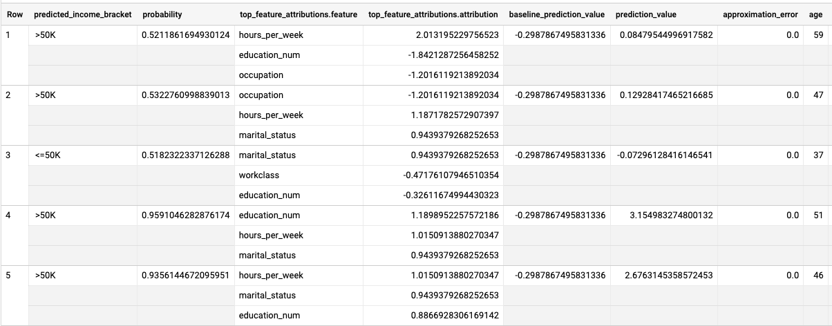
For logistic regression models, Shapley values are used to determine relative feature attribution for each feature in the model. Because the top_k_features option was set to 3 in the query, ML.EXPLAIN_PREDICT outputs the top three feature attributions for each row of the input_data view. These attributions are shown in descending order by the absolute value of the attribution.

Globally explain the model

To know which features are the most important to determine the income bracket, use the ML.GLOBAL_EXPLAIN function.

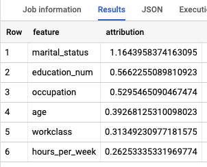
Get global explanations for the model:

1. In the Google Cloud console, go to the BigQuery page.

   Go to BigQuery

2. In the query editor, run the following query to get global explanations:

   SELECT
     *
   FROM
     ML.GLOBAL_EXPLAIN(MODEL `census.census_model`)

3. The results look similar to the following:

   

Clean up

To avoid incurring charges to your Google Cloud account for the resources used in this tutorial, either delete the project that contains the resources, or keep the project and delete the individual resources.

Delete your dataset

Deleting your project removes all datasets and all tables in the project. If you prefer to reuse the project, you can delete the dataset you created in this tutorial:

1. If necessary, open the BigQuery page in the Google Cloud console.

   Go to the BigQuery page

2. In the navigation, click the census dataset you created.

3. Click Delete dataset on the right side of the window. This action deletes the dataset and the model.

4. In the Delete dataset dialog, confirm the delete command by typing the name of your dataset (census) and then click Delete.

Delete your project

To delete the project:

Caution: Deleting a project has the following effects:

• Everything in the project is deleted. If you used an existing project for the tasks in this document, when you delete it, you also delete any other work you've done in the project.
• Custom project IDs are lost. When you created this project, you might have created a custom project ID that you want to use in the future. To preserve the URLs that use the project ID, such as an appspot.com URL, delete selected resources inside the project instead of deleting the whole project.

If you plan to explore multiple architectures, tutorials, or quickstarts, reusing projects can help you avoid exceeding project quota limits.

1. In the Google Cloud console, go to the Manage resources page.

   Go to Manage resources

2. In the project list, select the project that you want to delete, and then click Delete.
3. In the dialog, type the project ID, and then click Shut down to delete the project.

What's next

• For an overview of BigQuery ML, see Introduction to BigQuery ML.
• For information on creating models, see the CREATE MODEL syntax page.