在人口普查資料上建立及使用分類模型

---

在本教學課程中，您將在 BigQuery ML 中使用二元邏輯迴歸模型，根據個人的受眾特徵資料預測收入範圍。二元邏輯迴歸模型會預測某值是否屬於兩個類別之一，在本例中，即個人年收入是否超過或低於 $50,000 美元。

本教學課程使用 bigquery-public-data.ml_datasets.census_adult_income 資料集。這個資料集包含從 2000 年到 2010 年美國居民的人口和收入資訊。

目標

在本教學課程中，您將執行下列工作：

• 建立邏輯迴歸模型。
• 評估模型。
• 使用模型進行預測。
• 說明模型產生的結果。

費用

本教學課程使用 Google Cloud的計費元件，包括：

• BigQuery
• BigQuery ML

如要進一步瞭解 BigQuery 費用，請參閱 BigQuery 定價頁面。

如要進一步瞭解 BigQuery ML 費用，請參閱 BigQuery ML 定價。

事前準備

1. In the Google Cloud console, on the project selector page, select or create a Google Cloud project.

   Note: If you don't plan to keep the resources that you create in this procedure, create a project instead of selecting an existing project. After you finish these steps, you can delete the project, removing all resources associated with the project.

   Go to project selector

2. Verify that billing is enabled for your Google Cloud project.

3. Enable the BigQuery API.

   Enable the API

所需權限

如要使用 BigQuery ML 建立模型，您需要下列 IAM 權限：

• bigquery.jobs.create
• bigquery.models.create
• bigquery.models.getData
• bigquery.models.updateData
• bigquery.models.updateMetadata

如要執行推論，您需要下列權限：

• 模型上的 bigquery.models.getData
• bigquery.jobs.create

簡介

機器學習的常見工作是將資料分類為兩個類型 (稱為「標籤」) 之一。舉例來說，零售商可能會想要根據某個特定顧客的相關資訊，預測該顧客是否會購買某個新產品。在這種情況下，兩個標籤可能是 will buy 和 won't buy。零售商可以建構資料集，設定一個資料欄代表兩個標籤，並包含顧客資訊，例如顧客的位置、先前的購買內容和回報的偏好。零售商接著可以使用二元邏輯迴歸模型，根據這項顧客資訊預測最能代表每位顧客的標籤。

在本教學課程中，您將建立二元邏輯迴歸模型，根據受訪者的受眾特徵屬性，預測美國人口普查受訪者的收入是否屬於兩個範圍之一。

建立資料集

建立 BigQuery 資料集來儲存模型：

1. 前往 Google Cloud 控制台的「BigQuery」頁面。

   前往「BigQuery」

2. 在「Explorer」窗格中，按一下專案名稱。

3. 依序點按 「View actions」(查看動作) >「Create dataset」(建立資料集)。

4. 在「建立資料集」頁面中，執行下列操作：

   • 在「Dataset ID」(資料集 ID) 中輸入 census。

   • 針對「位置類型」選取「多區域」，然後選取「美國 (多個美國地區)」。

     公開資料集儲存在US 多地區。為簡單起見，請將資料集存放在相同位置。

   • 其餘設定請保留預設狀態，然後按一下「建立資料集」。

檢查資料

檢查資料集，然後找出要使用哪些資料欄做為邏輯迴歸模型的訓練資料。從 census_adult_income 資料表選取 100 列：

SQL

1. 前往 Google Cloud 控制台的「BigQuery」頁面。

   前往「BigQuery」

2. 在查詢編輯器中執行下列 GoogleSQL 查詢：

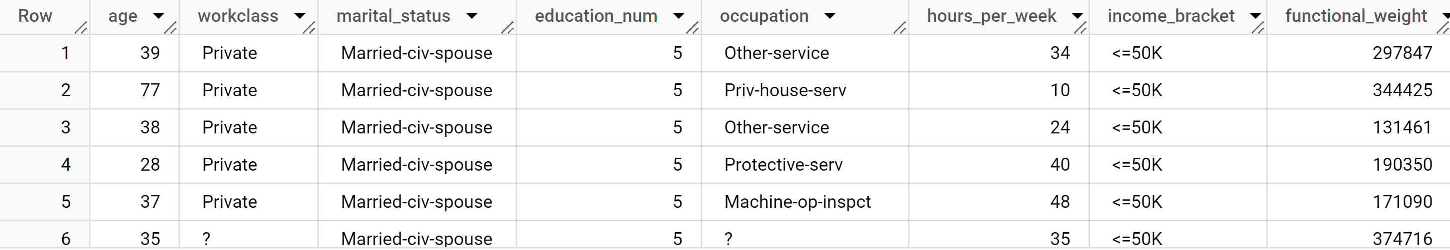
   SELECT
   age,
   workclass,
   marital_status,
   education_num,
   occupation,
   hours_per_week,
   income_bracket,
   functional_weight
   FROM
   `bigquery-public-data.ml_datasets.census_adult_income`
   LIMIT
   100;

3. 結果類似下方：

   

BigQuery DataFrames

在嘗試這個範例之前，請按照使用 BigQuery DataFrames 的 BigQuery 快速入門導覽課程中的 BigQuery DataFrames 設定說明操作。 詳情請參閱 BigQuery DataFrames 參考說明文件。

如要向 BigQuery 進行驗證，請設定應用程式預設憑證。 詳情請參閱「為本機開發環境設定 ADC」。

import bigframes.pandas as bpd

df = bpd.read_gbq(
    "bigquery-public-data.ml_datasets.census_adult_income",
    columns=(
        "age",
        "workclass",
        "marital_status",
        "education_num",
        "occupation",
        "hours_per_week",
        "income_bracket",
        "functional_weight",
    ),
    max_results=100,
)
df.peek()
# Output:
# age      workclass       marital_status  education_num          occupation  hours_per_week income_bracket  functional_weight
#  47      Local-gov   Married-civ-spouse             13      Prof-specialty              40           >50K             198660
#  56        Private        Never-married              9        Adm-clerical              40          <=50K              85018
#  40        Private   Married-civ-spouse             12        Tech-support              40           >50K             285787
#  34   Self-emp-inc   Married-civ-spouse              9        Craft-repair              54           >50K             207668
#  23        Private   Married-civ-spouse             10   Handlers-cleaners              40          <=50K              40060

查詢結果顯示 census_adult_income 資料表中的 income_bracket 資料欄只有以下兩個值其中之一：<=50K 或 >50K。

準備範例資料

在本教學課程中，您將根據 census_adult_income 表格中下列資料欄的值，預測人口普查受訪者的收入：

• age：受訪者的年齡。
• workclass：執行的工作類別。例如地方政府、私人或自營。
• marital_status
• education_num：受訪者的最高教育程度。
• occupation
• hours_per_week：每週工作時數。

排除重複資料的資料欄。舉例來說，education 資料欄，因為 education 和 education_num 資料欄值是以不同格式表達相同的資料。

functional_weight 資料欄是人口普查機構認為某個特定資料列所代表的個體數。由於這個資料欄的值與任何指定資料列的 income_bracket 值無關，因此您可以使用這個資料欄中的值，建立衍生自 functional_weight 資料欄的新 dataframe 資料欄，將資料分成訓練、評估和預測集。您會標記 80% 的資料用於訓練模型、10% 的資料用於評估，另外 10% 的資料則用於預測。

SQL

使用範例資料建立檢視畫面。本教學課程稍後的 CREATE MODEL 陳述式會使用這個檢視區塊。

執行查詢，準備範例資料：

1. 前往 Google Cloud 控制台的「BigQuery」頁面。

   前往「BigQuery」

2. 在查詢編輯器中執行下列查詢：

   CREATE OR REPLACE VIEW
   `census.input_data` AS
   SELECT
   age,
   workclass,
   marital_status,
   education_num,
   occupation,
   hours_per_week,
   income_bracket,
   CASE
     WHEN MOD(functional_weight, 10) < 8 THEN 'training'
     WHEN MOD(functional_weight, 10) = 8 THEN 'evaluation'
     WHEN MOD(functional_weight, 10) = 9 THEN 'prediction'
   END AS dataframe
   FROM
   `bigquery-public-data.ml_datasets.census_adult_income`;

3. 查看範例資料：

   SELECT * FROM `census.input_data`;

BigQuery DataFrames

建立名為 input_data 的 DataFrame。您會在後續步驟中使用 input_data 訓練模型、評估模型，以及進行預測。

在嘗試這個範例之前，請按照使用 BigQuery DataFrames 的 BigQuery 快速入門導覽課程中的 BigQuery DataFrames 設定說明操作。 詳情請參閱 BigQuery DataFrames 參考說明文件。

如要向 BigQuery 進行驗證，請設定應用程式預設憑證。 詳情請參閱「為本機開發環境設定 ADC」。

import bigframes.pandas as bpd

input_data = bpd.read_gbq(
    "bigquery-public-data.ml_datasets.census_adult_income",
    columns=(
        "age",
        "workclass",
        "marital_status",
        "education_num",
        "occupation",
        "hours_per_week",
        "income_bracket",
        "functional_weight",
    ),
)
input_data["dataframe"] = bpd.Series("training", index=input_data.index,).case_when(
    [
        (((input_data["functional_weight"] % 10) == 8), "evaluation"),
        (((input_data["functional_weight"] % 10) == 9), "prediction"),
    ]
)
del input_data["functional_weight"]

建立邏輯迴歸模型

使用您在前一節標記的訓練資料，建立邏輯迴歸模型。

SQL

使用 CREATE MODEL 陳述式，並指定模型類型為 LOGISTIC_REG。

以下是 CREATE MODEL 陳述式的重要資訊：

• input_label_cols 選項會指定 SELECT 陳述式中的哪個資料欄要當做標籤資料欄。這裡的標籤資料欄為 income_bracket，因此模型會根據特定資料列中呈現的其他值，學習 income_bracket 的兩個值中哪一個最有可能。

• 您不需要指定邏輯迴歸模型是二元或多重類別。BigQuery ML 會根據標籤資料欄中不重複值的數量，判斷要訓練哪種模型。

• auto_class_weights 選項會設為 TRUE，以平衡訓練資料中的類別標籤。預設情況下，訓練資料並未加權。如果訓練資料中的標籤不平衡，則模型學習到的權重可能不均，導致最熱門的標籤類別預測比例過高。在這種情況下，由於資料集中的大多數受訪者屬於較低的收入水平，所以模型預測較低收入水平的權重可能會因而過重。系統會透過與類別出現頻率成反比的方式，來計算每個類別的權重，藉此平衡各類別標籤的權重。

• enable_global_explain 選項設為 TRUE，讓您稍後在本教學課程中對模型使用 ML.GLOBAL_EXPLAIN 函式。

• SELECT 陳述式會查詢包含範例資料的 input_data 檢視區塊。WHERE 子句會篩選資料列，只有標示為訓練資料的資料列會用於訓練模型。

執行可建立邏輯迴歸模型的查詢：

1. 前往 Google Cloud 控制台的「BigQuery」頁面。

   前往「BigQuery」

2. 在查詢編輯器中執行下列查詢：

   CREATE OR REPLACE MODEL
   `census.census_model`
   OPTIONS
   ( model_type='LOGISTIC_REG',
     auto_class_weights=TRUE,
     enable_global_explain=TRUE,
     data_split_method='NO_SPLIT',
     input_label_cols=['income_bracket'],
     max_iterations=15) AS
   SELECT * EXCEPT(dataframe)
   FROM
   `census.input_data`
   WHERE
   dataframe = 'training'

3. 在「Explorer」窗格中，按一下「資料集」。

4. 在「資料集」窗格中，按一下 census。

5. 按一下「模型」窗格。

6. 按一下「census_model」。

7. 「詳細資料」分頁會列出 BigQuery ML 用來執行邏輯迴歸的屬性。

BigQuery DataFrames

使用 fit 方法訓練模型，並使用 to_gbq 方法將模型儲存至資料集。

在嘗試這個範例之前，請按照使用 BigQuery DataFrames 的 BigQuery 快速入門導覽課程中的 BigQuery DataFrames 設定說明操作。 詳情請參閱 BigQuery DataFrames 參考說明文件。

如要向 BigQuery 進行驗證，請設定應用程式預設憑證。 詳情請參閱「為本機開發環境設定 ADC」。

import bigframes.ml.linear_model

# input_data is defined in an earlier step.
training_data = input_data[input_data["dataframe"] == "training"]
X = training_data.drop(columns=["income_bracket", "dataframe"])
y = training_data["income_bracket"]

census_model = bigframes.ml.linear_model.LogisticRegression(
    # Balance the class labels in the training data by setting
    # class_weight="balanced".
    #
    # By default, the training data is unweighted. If the labels
    # in the training data are imbalanced, the model may learn to
    # predict the most popular class of labels more heavily. In
    # this case, most of the respondents in the dataset are in the
    # lower income bracket. This may lead to a model that predicts
    # the lower income bracket too heavily. Class weights balance
    # the class labels by calculating the weights for each class in
    # inverse proportion to the frequency of that class.
    class_weight="balanced",
    max_iterations=15,
)
census_model.fit(X, y)

census_model.to_gbq(
    your_model_id,  # For example: "your-project.census.census_model"
    replace=True,
)

評估模型成效

建立模型後，請根據評估資料評估模型成效。

SQL

ML.EVALUATE 函式會根據評估資料，評估模型產生的預測值。

ML.EVALUATE 函式會將訓練好的模型和 input_data 檢視畫面中的資料列做為輸入內容，這些資料列的 dataframe 資料欄值為 evaluation。該函式會傳回模型相關統計資料的單一資料列。

執行 ML.EVALUATE 查詢：

1. 前往 Google Cloud 控制台的「BigQuery」頁面。

   前往「BigQuery」

2. 在查詢編輯器中執行下列查詢：

   SELECT
   *
   FROM
   ML.EVALUATE (MODEL `census.census_model`,
     (
     SELECT
       *
     FROM
       `census.input_data`
     WHERE
       dataframe = 'evaluation'
     )
   );

3. 結果類似下方：

   

BigQuery DataFrames

使用 score 方法，根據實際資料評估模型。

在嘗試這個範例之前，請按照使用 BigQuery DataFrames 的 BigQuery 快速入門導覽課程中的 BigQuery DataFrames 設定說明操作。 詳情請參閱 BigQuery DataFrames 參考說明文件。

如要向 BigQuery 進行驗證，請設定應用程式預設憑證。 詳情請參閱「為本機開發環境設定 ADC」。

# Select model you'll use for predictions. `read_gbq_model` loads model
# data from BigQuery, but you could also use the `census_model` object
# from previous steps.
census_model = bpd.read_gbq_model(
    your_model_id,  # For example: "your-project.census.census_model"
)

# input_data is defined in an earlier step.
evaluation_data = input_data[input_data["dataframe"] == "evaluation"]
X = evaluation_data.drop(columns=["income_bracket", "dataframe"])
y = evaluation_data["income_bracket"]

# The score() method evaluates how the model performs compared to the
# actual data. Output DataFrame matches that of ML.EVALUATE().
score = census_model.score(X, y)
score.peek()
# Output:
#    precision    recall  accuracy  f1_score  log_loss   roc_auc
# 0   0.685764  0.536685   0.83819  0.602134  0.350417  0.882953

您也可以在 Google Cloud 控制台中查看模型的「評估」窗格，瞭解訓練期間計算的評估指標：

預測收入級距

使用模型預測每位受訪者最有可能的收入水平。

SQL

使用 ML.PREDICT 函式預測可能的收入水平。做為輸入內容，ML.PREDICT 函式會採用訓練好的模型，以及 dataframe 資料欄值為 prediction 的 input_data 檢視畫面中的資料列。

執行 ML.PREDICT 查詢：

1. 前往 Google Cloud 控制台的「BigQuery」頁面。

   前往「BigQuery」

2. 在查詢編輯器中執行下列查詢：

   SELECT
   *
   FROM
   ML.PREDICT (MODEL `census.census_model`,
     (
     SELECT
       *
     FROM
       `census.input_data`
     WHERE
       dataframe = 'prediction'
     )
   );

3. 結果類似下方：

   

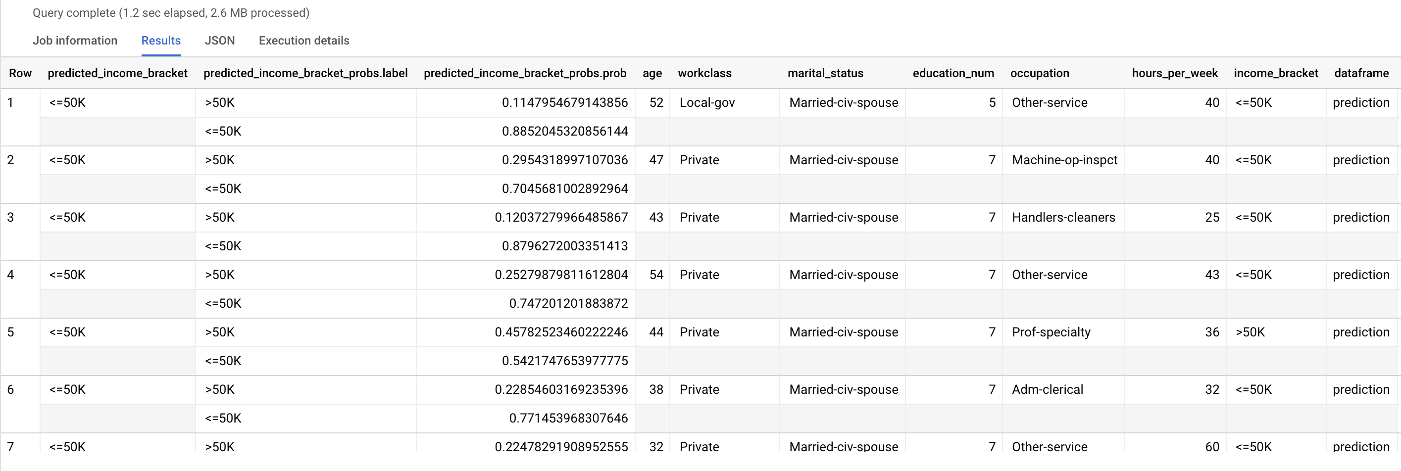
predicted_income_bracket 欄包含受訪者的預測收入水平。

BigQuery DataFrames

使用 predict 方法預測可能的所得級距。

在嘗試這個範例之前，請按照使用 BigQuery DataFrames 的 BigQuery 快速入門導覽課程中的 BigQuery DataFrames 設定說明操作。 詳情請參閱 BigQuery DataFrames 參考說明文件。

如要向 BigQuery 進行驗證，請設定應用程式預設憑證。 詳情請參閱「為本機開發環境設定 ADC」。

# Select model you'll use for predictions. `read_gbq_model` loads model
# data from BigQuery, but you could also use the `census_model` object
# from previous steps.
census_model = bpd.read_gbq_model(
    your_model_id,  # For example: "your-project.census.census_model"
)

# input_data is defined in an earlier step.
prediction_data = input_data[input_data["dataframe"] == "prediction"]

predictions = census_model.predict(prediction_data)
predictions.peek()
# Output:
#           predicted_income_bracket                     predicted_income_bracket_probs  age workclass  ... occupation  hours_per_week income_bracket   dataframe
# 18004                    <=50K  [{'label': ' >50K', 'prob': 0.0763305999358786...   75         ?  ...          ?               6          <=50K  prediction
# 18886                    <=50K  [{'label': ' >50K', 'prob': 0.0448866871906495...   73         ?  ...          ?              22           >50K  prediction
# 31024                    <=50K  [{'label': ' >50K', 'prob': 0.0362982319421936...   69         ?  ...          ?               1          <=50K  prediction
# 31022                    <=50K  [{'label': ' >50K', 'prob': 0.0787836112058324...   75         ?  ...          ?               5          <=50K  prediction
# 23295                    <=50K  [{'label': ' >50K', 'prob': 0.3385373037905673...   78         ?  ...          ?              32          <=50K  prediction

說明預測結果

如要瞭解模型產生這些預測結果的原因，可以使用 ML.EXPLAIN_PREDICT 函式。

ML.EXPLAIN_PREDICT 是 ML.PREDICT 函式的擴充版本。 ML.EXPLAIN_PREDICT 不僅會輸出預測結果，也會輸出額外資料欄來解釋預測結果。如要進一步瞭解可解釋性，請參閱 BigQuery ML 可解釋性 AI 總覽。

執行 ML.EXPLAIN_PREDICT 查詢：

1. 前往 Google Cloud 控制台的「BigQuery」頁面。

   前往「BigQuery」

2. 在查詢編輯器中執行下列查詢：

   SELECT
   *
   FROM
   ML.EXPLAIN_PREDICT(MODEL `census.census_model`,
     (
     SELECT
       *
     FROM
       `census.input_data`
     WHERE
       dataframe = 'evaluation'),
     STRUCT(3 as top_k_features));

3. 結果類似下方：

   

注意： ML.EXPLAIN_PREDICT 查詢會輸出所有輸入特徵資料欄，與 ML.PREDICT 的做法類似。為方便閱讀，上圖只顯示一個特徵資料欄 age。

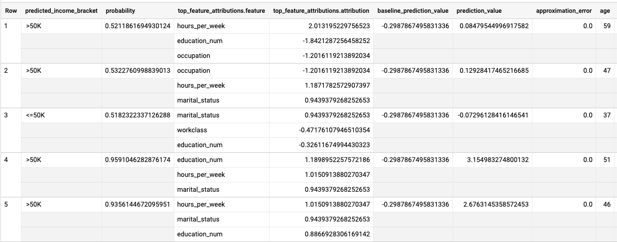
對於邏輯迴歸模型，系統會使用 Shapley 值，判斷模型中每個特徵的相對特徵歸因。由於查詢中的 top_k_features 選項設為 3，因此 ML.EXPLAIN_PREDICT 會輸出 input_data 檢視表中每個資料列的前三項特徵屬性。這些歸因會依歸因絕對值遞減排序。

從全域角度說明模型

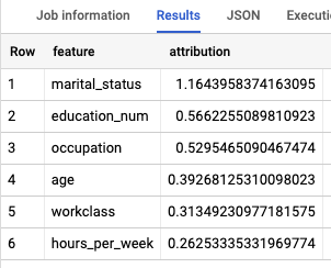
如要瞭解哪些特徵最重要，可決定收入水平，請使用 ML.GLOBAL_EXPLAIN 函式。

取得模型的全域說明：

1. 前往 Google Cloud 控制台的「BigQuery」頁面。

   前往「BigQuery」

2. 在查詢編輯器中執行下列查詢，取得全域說明：

   SELECT
     *
   FROM
     ML.GLOBAL_EXPLAIN(MODEL `census.census_model`)

3. 結果類似下方：

   

清除所用資源

如要避免系統向您的 Google Cloud 帳戶收取本教學課程中所用資源的相關費用，請刪除含有該項資源的專案，或者保留專案但刪除個別資源。

刪除資料集

刪除專案將移除專案中所有的資料集與資料表。若您希望重新使用專案，您可以刪除本教學課程中所建立的資料集。

1. 如有必要，請在Google Cloud 控制台中開啟 BigQuery 頁面。

   前往 BigQuery 頁面

2. 在導覽窗格中，按一下您建立的 census 資料集。

3. 按一下視窗右側的「刪除資料集」。 這個動作會刪除資料集和模型。

4. 在「Delete dataset」(刪除資料集) 對話方塊中，輸入資料集的名稱 (census)，然後按一下「Delete」(刪除) 來確認刪除指令。

刪除專案

如要刪除專案，請進行以下操作：

注意：刪除專案會造成以下結果：

• 專案中的所有內容都會遭到刪除。 如果您使用現有專案來進行本文中的工作，刪除專案將一併刪除其中已完成的所有工作。
• 自訂的專案 ID 會消失。當您之前建立這個專案時，可能建立了想要在日後使用的自訂專案 ID。如要保留使用該專案 ID 的網址 (例如 appspot.com 網址)，請刪除在該專案中選取的資源，而不是刪除整個專案。

如果打算探索多種架構、教學課程或快速入門導覽課程，重複使用專案有助於避免超出專案配額限制。

1. In the Google Cloud console, go to the Manage resources page.

   Go to Manage resources

2. In the project list, select the project that you want to delete, and then click Delete.
3. In the dialog, type the project ID, and then click Shut down to delete the project.

後續步驟

• 如需 BigQuery ML 的總覽，請參閱 BigQuery ML 簡介。
• 如要瞭解如何建立模型，請參閱 CREATE MODEL 語法頁面。