在本教學課程中,您將使用 Colab 筆記本,以視覺化方式呈現 BigQuery 的地理空間分析資料。
本教學課程使用下列 BigQuery 公開資料集:
如要瞭解如何存取這些公開資料集,請參閱「在 Google Cloud 控制台中存取公開資料集」。
您可以使用公開資料集建立下列視覺化效果:
- Ford GoBike Share 資料集的所有共享單車站點散佈圖
- 舊金山社區資料集中的多邊形
- 按社區劃分的共享單車站數量等值線圖
- 舊金山警察局報告資料集的事件熱度圖
建立 Colab 筆記本
本教學課程會建立 Colab 筆記本,以視覺化方式呈現地理空間分析資料。如要在 Colab、Colab Enterprise 或 BigQuery Studio 中開啟筆記本的預先建構版本,請按一下教學課程 GitHub 版本頂端的連結「BigQuery Geospatial Visualization in Colab」(在 Colab 中進行 BigQuery 地理空間資料視覺化)。
開啟 Colab。
在「開啟筆記本」對話方塊中,按一下「新增筆記本」。
按一下
Untitled0.ipynb,然後將筆記本名稱變更為bigquery-geo.ipynb。依序選取「檔案」>「儲存」。
使用 Google Cloud 和 Google 地圖進行驗證
本教學課程會查詢 BigQuery 資料集,並使用 Google 地圖 JavaScript API。如要使用這些資源,請透過 Google Cloud 和 Maps API 驗證 Colab 執行階段。
透過 Google Cloud驗證
如要插入程式碼儲存格,請按一下 「程式碼」。
如要使用專案進行驗證,請輸入下列程式碼:
# REQUIRED: Authenticate with your project.
GCP_PROJECT_ID = "PROJECT_ID"  #@param {type:"string"}

from google.colab import auth
from google.colab import userdata

auth.authenticate_user(project_id=GCP_PROJECT_ID)

# Set GMP_API_KEY to none
GMP_API_KEY = None
將 PROJECT_ID 替換為您的專案 ID。
按一下 「執行儲存格」。
出現提示時,請按一下「允許」,同意授予 Colab 憑證存取權。
在「使用 Google 帳戶登入」頁面中,選擇您的帳戶。
在「Sign in to Third-party authored notebook code」(登入第三方撰寫的筆記本程式碼) 頁面中,按一下「Continue」(繼續)。
在「選取第三方撰寫的筆記本程式碼可存取哪些項目」頁面,按一下「全選」,然後點選「繼續」。
完成授權流程後,Colab 筆記本不會產生任何輸出內容。儲存格旁的勾號表示程式碼已順利執行。
選用:使用 Google 地圖驗證
如果您使用 Google 地圖平台做為基本地圖的地圖供應商,請務必提供 Google 地圖平台 API 金鑰。筆記本會從 Colab 密鑰擷取金鑰。
如果您使用 Maps API,才需要執行這個步驟。如果沒有透過 Google 地圖平台進行驗證,pydeck 會改用 carto 地圖。
按照 Google 地圖說明文件「使用 API 金鑰」頁面的操作說明,取得 Google Maps API 金鑰。
切換至 Colab 筆記本,然後按一下「密碼」。
按一下「新增密碼」。
在「Name」(名稱) 中輸入
GMP_API_KEY。在「Value」部分輸入先前產生的 Maps API 金鑰值。
關閉「密鑰」面板。
如要插入程式碼儲存格,請按一下 「程式碼」。
如要透過 Maps API 進行驗證,請輸入下列程式碼:
# Authenticate with the Google Maps JavaScript API.
GMP_API_SECRET_KEY_NAME = "GMP_API_KEY" #@param {type:"string"}

if GMP_API_SECRET_KEY_NAME:
  GMP_API_KEY = userdata.get(GMP_API_SECRET_KEY_NAME) if GMP_API_SECRET_KEY_NAME else None
else:
  GMP_API_KEY = None
如果同意,請在系統提示時按一下「授予存取權」,讓筆記本存取您的金鑰。
按一下 「執行儲存格」。
完成授權流程後,Colab 筆記本不會產生任何輸出內容。儲存格旁的勾號表示程式碼已順利執行。
安裝 Python 套件並匯入資料科學程式庫
除了 colabtools (google.colab) Python 模組,本教學課程還會使用其他 Python 套件和資料科學程式庫。
在本節中,您將安裝 pydeck 和 h3 套件。pydeck
提供以 deck.gl 為基礎的 Python 大規模空間算繪功能。
h3-py 提供 Python 版的 Uber H3 六邊形階層式地理空間索引系統。
接著匯入 h3 和 pydeck 程式庫,以及下列 Python 地理空間程式庫:
geopandas擴充pandas使用的資料類型,允許對幾何類型執行空間作業。shapely,用於操控和分析個別平面幾何物件。branca,產生 HTML 和 JavaScript 色彩對應。geemap.deck使用pydeck和earthengine-api進行視覺化。
匯入程式庫後,請為 pandas Colab 中的 DataFrame 啟用互動式表格。
安裝 pydeck 和 h3 套件
如要插入程式碼儲存格,請按一下 「程式碼」。
如要安裝
pydeck和h3套件,請輸入下列程式碼:# Install pydeck and h3. !pip install pydeck>=0.9 h3>=4.2
按一下 「執行儲存格」。
安裝完成後,Colab 筆記本不會產生任何輸出內容。儲存格旁的勾號表示程式碼已順利執行。
匯入 Python 程式庫
如要插入程式碼儲存格,請按一下 「程式碼」。
如要匯入 Python 程式庫,請輸入下列程式碼:
# Import data science libraries.
import branca
import geemap.deck as gmdk
import h3
import pydeck as pdk
import geopandas as gpd
import shapely
按一下 「執行儲存格」。
執行程式碼後,Colab 筆記本不會產生任何輸出內容。儲存格旁的勾號表示程式碼已順利執行。
為 pandas DataFrame 啟用互動式表格
如要插入程式碼儲存格,請按一下 「程式碼」。
如要啟用
pandasDataFrame,請輸入下列程式碼:# Enable displaying pandas data frames as interactive tables by default. from google.colab import data_table data_table.enable_dataframe_formatter()
按一下 「執行儲存格」。
執行程式碼後,Colab 筆記本不會產生任何輸出內容。儲存格旁的勾號表示程式碼已順利執行。
建立共用處理常式
在本節中,您會建立共用常式,在基本地圖上算繪圖層。
如要插入程式碼儲存格,請按一下 「程式碼」。
如要建立共用常式,在 Google 地圖上算繪圖層,請輸入下列程式碼:
# Set Google Maps as the base map provider.
MAP_PROVIDER_GOOGLE = pdk.bindings.base_map_provider.BaseMapProvider.GOOGLE_MAPS.value

# Shared routine for rendering layers on a map using geemap.deck.
def display_pydeck_map(layers, view_state, **kwargs):
  deck_kwargs = kwargs.copy()

  # Use Google Maps as the base map only if the API key is provided.
  if GMP_API_KEY:
    deck_kwargs.update({
      "map_provider": MAP_PROVIDER_GOOGLE,
      "map_style": pdk.bindings.map_styles.GOOGLE_ROAD,
      "api_keys": {MAP_PROVIDER_GOOGLE: GMP_API_KEY},
    })

  m = gmdk.Map(initial_view_state=view_state, ee_initialize=False, **deck_kwargs)

  for layer in layers:
    m.add_layer(layer)
  return m
按一下 「執行儲存格」。
執行程式碼後,Colab 筆記本不會產生任何輸出內容。儲存格旁的勾號表示程式碼已順利執行。
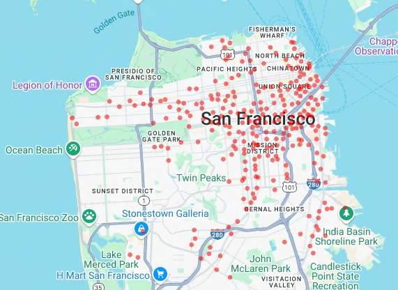
建立散布圖
在本節中,您將從 bigquery-public-data.san_francisco_bikeshare.bikeshare_station_info 資料表擷取資料,建立舊金山 Ford GoBike Share 公開資料集中所有共享單車站的散佈圖。散布圖是使用 deck.gl 架構中的圖層和散布圖層建立。
當您需要查看個別點的子集 (也稱為抽查) 時,散佈圖就派得上用場。
以下範例說明如何使用圖層和散佈圖層,將個別點算繪為圓圈。
如要插入程式碼儲存格,請按一下 「程式碼」。
如要查詢舊金山 Ford GoBike Share 公開資料集,請輸入下列程式碼。這段程式碼使用
%%bigquery神奇函式執行查詢,並以 DataFrame 形式傳回結果:# Query the station ID, station name, station short name, and station # geometry from the bike share dataset. # NOTE: In this tutorial, the denormalized 'lat' and 'lon' columns are # ignored. They are decomposed components of the geometry. %%bigquery gdf_sf_bikestations --project {GCP_PROJECT_ID} --use_geodataframe station_geom SELECT station_id, name, short_name, station_geom FROM `bigquery-public-data.san_francisco_bikeshare.bikeshare_station_info`
按一下 「執行儲存格」。
輸出結果會與下列內容相似:
Job ID 12345-1234-5678-1234-123456789 successfully executed: 100%如要插入程式碼儲存格,請按一下 「程式碼」。
如要取得 DataFrame 的摘要 (包括資料欄和資料類型),請輸入下列程式碼:
# Get a summary of the DataFrame
gdf_sf_bikestations.info()
按一下 「執行儲存格」。
輸出內容應如下所示:
<class 'geopandas.geodataframe.GeoDataFrame'>
RangeIndex: 472 entries, 0 to 471
Data columns (total 4 columns):
#   Column        Non-Null Count  Dtype
---  ------        --------------  -----
0   station_id    472 non-null    object
1   name          472 non-null    object
2   short_name    472 non-null    object
3   station_geom  472 non-null    geometry
dtypes: geometry(1), object(3)
memory usage: 14.9+ KB
如要插入程式碼儲存格,請按一下 「程式碼」。
如要預覽 DataFrame 的前五列,請輸入下列程式碼:
# Preview the first five rows
gdf_sf_bikestations.head()
按一下 「執行儲存格」。
輸出結果會與下列內容相似:
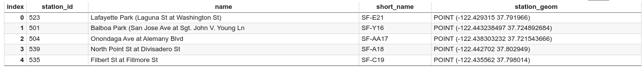
如要轉譯點,必須從單車共乘資料集的 station_geom 欄位中,將經緯度擷取為 x 和 y 座標。
由於 gdf_sf_bikestations 是 geopandas.GeoDataFrame,因此可直接從其 station_geom 幾何圖形欄存取座標。您可以使用資料欄的 .x 屬性擷取經度,並使用 .y 屬性擷取緯度。然後儲存在新的經緯度欄中。
如要插入程式碼儲存格,請按一下 「程式碼」。
如要從「
station_geom」欄擷取經緯度值,請輸入下列程式碼:# Extract the longitude (x) and latitude (y) from station_geom. gdf_sf_bikestations["longitude"] = gdf_sf_bikestations["station_geom"].x gdf_sf_bikestations["latitude"] = gdf_sf_bikestations["station_geom"].y
按一下 「執行儲存格」。
執行程式碼後,Colab 筆記本不會產生任何輸出內容。儲存格旁的勾號表示程式碼已順利執行。
如要插入程式碼儲存格,請按一下 「程式碼」。
如要根據先前擷取的經緯度值,算繪自行車共享站的散佈圖,請輸入下列程式碼:
# Render a scatter plot using pydeck with the extracted longitude and
# latitude columns in the gdf_sf_bikestations geopandas.GeoDataFrame.
scatterplot_layer = pdk.Layer(
  "ScatterplotLayer",
  id="bike_stations_scatterplot",
  data=gdf_sf_bikestations,
  get_position=['longitude', 'latitude'],
  get_radius=100,
  get_fill_color=[255, 0, 0, 140],  # Adjust color as desired
  pickable=True,
)

view_state = pdk.ViewState(latitude=37.77613, longitude=-122.42284, zoom=12)
display_pydeck_map([scatterplot_layer], view_state)
按一下 「執行儲存格」。
輸出結果會與下列內容相似:
顯示多邊形
地理空間分析功能可讓您使用 GEOGRAPHY 資料類型和 GoogleSQL 地理函式,在 BigQuery 中分析及視覺化呈現地理空間資料。
地理空間分析中的 GEOGRAPHY 資料型別是點、線串和多邊形的集合,以地球表面的點集合或子集合表示。GEOGRAPHY 型別可包含下列物件:
- 資料點
- 線條
- 多邊形
- 多邊形集合
如需所有支援物件的清單,請參閱 GEOGRAPHY 類型說明文件。
如果您取得地理空間資料,但不知道預期形狀,可以將資料視覺化,找出形狀。您可以將地理資料轉換為 GeoJSON 格式,以視覺化呈現形狀。然後,您可以使用 deck.gl 架構中的 GeoJSON 圖層,將 GeoJSON 資料視覺化。
在本節中,您將查詢舊金山鄰近地區資料集中的地理資料,然後以視覺化方式呈現多邊形。
如要插入程式碼儲存格,請按一下 「程式碼」。
如要查詢「舊金山鄰近地區」資料集
bigquery-public-data.san_francisco_neighborhoods.boundaries資料表中的地理資料,請輸入下列程式碼。這段程式碼會使用%%bigquerymagic 函式執行查詢,並以 DataFrame 形式傳回結果:# Query the neighborhood name and geometry from the San Francisco # neighborhoods dataset. %%bigquery gdf_sanfrancisco_neighborhoods --project {GCP_PROJECT_ID} --use_geodataframe geometry SELECT neighborhood, neighborhood_geom AS geometry FROM `bigquery-public-data.san_francisco_neighborhoods.boundaries`
按一下 「執行儲存格」。
輸出結果會與下列內容相似:
Job ID 12345-1234-5678-1234-123456789 successfully executed: 100%如要插入程式碼儲存格,請按一下 「程式碼」。
如要取得 DataFrame 的摘要,請輸入下列程式碼:
# Get a summary of the DataFrame
gdf_sanfrancisco_neighborhoods.info()
按一下 「執行儲存格」。
結果應如下所示:
<class 'geopandas.geodataframe.GeoDataFrame'>
RangeIndex: 117 entries, 0 to 116
Data columns (total 2 columns):
#   Column        Non-Null Count  Dtype
---  ------        --------------  -----
0   neighborhood  117 non-null    object
1   geometry      117 non-null    geometry
dtypes: geometry(1), object(1)
memory usage: 2.0+ KB
如要預覽 DataFrame 的第一列,請輸入下列程式碼:
# Preview the first row
gdf_sanfrancisco_neighborhoods.head(1)
按一下 「執行儲存格」。
輸出結果會與下列內容相似:
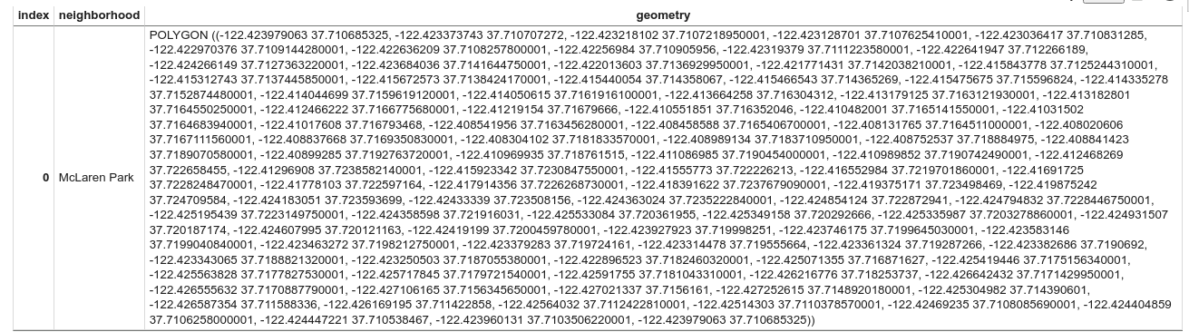
在結果中,請注意資料是多邊形。
如要插入程式碼儲存格,請按一下 「程式碼」。
如要將多邊形視覺化,請輸入下列程式碼。
pydeck用於將幾何資料欄中的每個shapely物件例項轉換為GeoJSON格式:# Visualize the polygons. geojson_layer = pdk.Layer( 'GeoJsonLayer', id="sf_neighborhoods", data=gdf_sanfrancisco_neighborhoods, get_line_color=[127, 0, 127, 255], get_fill_color=[60, 60, 60, 50], get_line_width=100, pickable=True, stroked=True, filled=True, ) view_state = pdk.ViewState(latitude=37.77613, longitude=-122.42284, zoom=12) display_pydeck_map([geojson_layer], view_state)
按一下 「執行儲存格」。
輸出結果會與下列內容相似:
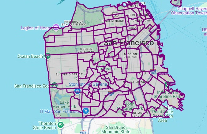
製作 choropleth 地圖
如果您要探索的資料包含難以轉換為 GeoJSON 格式的多邊形,可以改用 deck.gl 架構的多邊形圖層。多邊形圖層可以處理特定類型的輸入資料,例如點陣列。
在本節中,您將使用多邊形圖層算繪點陣列,並使用結果算繪 choropleth 地圖。等值線地圖會結合「舊金山鄰近地區」資料集和「舊金山 Ford GoBike 共享單車」資料集中的資料,顯示各鄰近地區的共享單車站密度。
如要插入程式碼儲存格,請按一下 「程式碼」。
如要匯總及計算每個社區的電台數量,並建立包含點陣列的
polygon欄,請輸入下列程式碼:# Aggregate and count the number of stations per neighborhood. gdf_count_stations = gdf_sanfrancisco_neighborhoods.sjoin(gdf_sf_bikestations, how='left', predicate='contains') gdf_count_stations = gdf_count_stations.groupby(by='neighborhood')['station_id'].count().rename('num_stations') gdf_stations_x_neighborhood = gdf_sanfrancisco_neighborhoods.join(gdf_count_stations, on='neighborhood', how='inner') # To simulate non-GeoJSON input data, create a polygon column that contains # an array of points by using the pandas.Series.map method. gdf_stations_x_neighborhood['polygon'] = gdf_stations_x_neighborhood['geometry'].map(lambda g: list(g.exterior.coords))
按一下 「執行儲存格」。
執行程式碼後,Colab 筆記本不會產生任何輸出內容。儲存格旁的勾號表示程式碼已順利執行。
如要插入程式碼儲存格,請按一下 「程式碼」。
如要為每個多邊形新增
fill_color欄,請輸入下列程式碼:# Create a color map gradient using the branch library, and add a fill_color # column for each of the polygons. colormap = branca.colormap.LinearColormap( colors=["lightblue", "darkred"], vmin=0, vmax=gdf_stations_x_neighborhood['num_stations'].max(), ) gdf_stations_x_neighborhood['fill_color'] = gdf_stations_x_neighborhood['num_stations'] \ .map(lambda c: list(colormap.rgba_bytes_tuple(c)[:3]) + [0.7 * 255]) # force opacity of 0.7
按一下 「執行儲存格」。
執行程式碼後,Colab 筆記本不會產生任何輸出內容。儲存格旁的勾號表示程式碼已順利執行。
如要插入程式碼儲存格,請按一下 「程式碼」。
如要算繪多邊形圖層,請輸入下列程式碼:
# Render the polygon layer.
polygon_layer = pdk.Layer(
  'PolygonLayer',
  id="bike_stations_choropleth",
  data=gdf_stations_x_neighborhood,
  get_polygon='polygon',
  get_fill_color='fill_color',
  get_line_color=[0, 0, 0, 255],
  get_line_width=50,
  pickable=True,
  stroked=True,
  filled=True,
)
view_state = pdk.ViewState(latitude=37.77613, longitude=-122.42284, zoom=12)
display_pydeck_map([polygon_layer], view_state)
按一下 「執行儲存格」。
輸出結果會與下列內容相似:
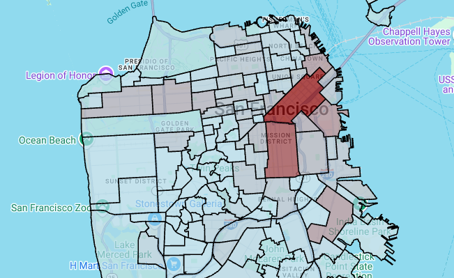
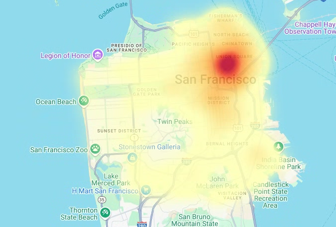
建立熱視圖
如果您有已知的有意義界線,就適合使用等值線圖。如果資料沒有已知的有意義界線,可以使用熱度圖層算繪連續密度。
在以下範例中,您會查詢舊金山警察局 (SFPD) 報告資料集內 bigquery-public-data.san_francisco_sfpd_incidents.sfpd_incidents 資料表中的資料。這些資料用於呈現 2015 年事件的分布情形。
如果是熱視圖,建議您先量化及彙整資料,再進行算繪。在本例中,資料會使用 Carto H3 空間索引進行量化和匯總。熱視圖是使用 deck.gl 架構的熱視圖圖層建立。
在本範例中,量化作業是使用 h3 Python 程式庫,將事件點匯總到六邊形中。h3.latlng_to_cell 函式用於將事件的位置 (緯度和經度) 對應至 H3 儲存格索引。九的 H3 解析度可提供足夠的聚合六邊形,用於熱度圖。h3.cell_to_latlng 函式用於判斷每個六邊形的中心。
如要插入程式碼儲存格,請按一下 「程式碼」。
如要查詢舊金山警察局 (SFPD) 報告資料集中的資料,請輸入下列程式碼。這段程式碼會使用
%%bigquerymagic 函式執行查詢,並以 DataFrame 形式傳回結果:# Query the incident key and location data from the SFPD reports dataset. %%bigquery gdf_incidents --project {GCP_PROJECT_ID} --use_geodataframe location_geography SELECT unique_key, location_geography FROM ( SELECT unique_key, SAFE.ST_GEOGFROMTEXT(location) AS location_geography, # WKT string to GEOMETRY EXTRACT(YEAR FROM timestamp) AS year, FROM `bigquery-public-data.san_francisco_sfpd_incidents.sfpd_incidents` incidents ) WHERE year = 2015
按一下 「執行儲存格」。
輸出結果會與下列內容相似:
Job ID 12345-1234-5678-1234-123456789 successfully executed: 100%如要插入程式碼儲存格,請按一下 「程式碼」。
如要計算每個事件的經緯度儲存格,請匯總每個儲存格的事件、建構
geopandasDataFrame,並為熱度圖層新增每個六邊形的中心,然後輸入下列程式碼:# Compute the cell for each incident's latitude and longitude. H3_RESOLUTION = 9 gdf_incidents['h3_cell'] = gdf_incidents.geometry.apply( lambda geom: h3.latlng_to_cell(geom.y, geom.x, H3_RESOLUTION) ) # Aggregate the incidents for each hexagon cell. count_incidents = gdf_incidents.groupby(by='h3_cell')['unique_key'].count().rename('num_incidents') # Construct a new geopandas.GeoDataFrame with the aggregate results. # Add the center of each hexagon for the HeatmapLayer to render. gdf_incidents_x_cell = gpd.GeoDataFrame(data=count_incidents).reset_index() gdf_incidents_x_cell['h3_center'] = gdf_incidents_x_cell['h3_cell'].apply(h3.cell_to_latlng) gdf_incidents_x_cell.info()
按一下 「執行儲存格」。
輸出結果會與下列內容相似:
<class 'geopandas.geodataframe.GeoDataFrame'>
RangeIndex: 969 entries, 0 to 968
Data columns (total 3 columns):
#   Column         Non-Null Count  Dtype
--  ------         --------------  -----
0   h3_cell        969 non-null    object
1   num_incidents  969 non-null    Int64
2   h3_center      969 non-null    object
dtypes: Int64(1), object(2)
memory usage: 23.8+ KB
如要插入程式碼儲存格,請按一下 「程式碼」。
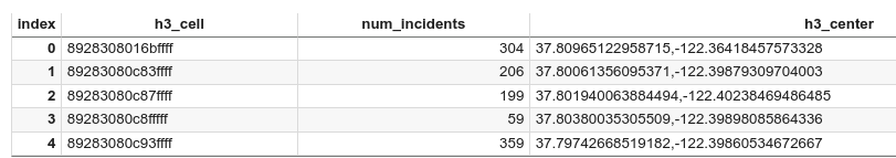
如要預覽 DataFrame 的前五列,請輸入下列程式碼:
# Preview the first five rows.
gdf_incidents_x_cell.head()
按一下 「執行儲存格」。
輸出結果會與下列內容相似:
如要插入程式碼儲存格,請按一下 「程式碼」。
如要將資料轉換為
HeatmapLayer可用的 JSON 格式,請輸入下列程式碼:# Convert to a JSON format recognized by the HeatmapLayer. def _make_heatmap_datum(row) -> dict: return { "latitude": row['h3_center'][0], "longitude": row['h3_center'][1], "weight": float(row['num_incidents']), } heatmap_data = gdf_incidents_x_cell.apply(_make_heatmap_datum, axis='columns').values.tolist()
按一下 「執行儲存格」。
執行程式碼後,Colab 筆記本不會產生任何輸出內容。儲存格旁的勾號表示程式碼已順利執行。
如要插入程式碼儲存格,請按一下 「程式碼」。
如要算繪熱度圖,請輸入下列程式碼:
# Render the heatmap.
heatmap_layer = pdk.Layer(
  "HeatmapLayer",
  id="sfpd_heatmap",
  data=heatmap_data,
  get_position=['longitude', 'latitude'],
  get_weight='weight',
  opacity=0.7,
  radius_pixels=99,  # this limitation can introduce artifacts (see above)
  aggregation='MEAN',
)
view_state = pdk.ViewState(latitude=37.77613, longitude=-122.42284, zoom=12)
display_pydeck_map([heatmap_layer], view_state)
按一下 「執行儲存格」。
輸出結果會與下列內容相似: