Machine learning models are often "black boxes"; even their designers cannot explain how or why a model produced a specific inference. Vertex Explainable AI offers Feature-based and Example-based explanations to provide better understanding of model decision making.
Knowing how a model behaves, and how its training dataset influences the model, gives anyone who builds or uses ML new abilities to improve models, build confidence in their inferences, and understand when and why things go awry.
Example-based explanations
With example-based explanations, Vertex AI uses nearest neighbor search to return a list of examples (typically from the training set) that are most similar to the input. Because we generally expect similar inputs to yield similar inferences, we can use these explanations to explore and explain our model's behavior.
Example-based explanations can be useful in several scenarios:
Improve your data or model: One of the core use cases for example-based explanations is helping you understand why your model made certain mistakes in its inferences, and using those insights to improve your data or model. To do so, first select test data that is of interest to you. This could be either driven by business needs or heuristics like data where the model made the most egregious mistakes.
For example, suppose we have a model that classifies images as either a bird or a plane and misclassifies the following bird as a plane with high confidence. Use Example-based explanations to retrieve similar images from the training set to figure out what is happening.

Since all of its explanations are dark silhouettes from the plane class, it's a signal to get more bird silhouettes.
However, if the explanations were mainly from the bird class, it's a signal that our model can't learn relationships even when the data is rich, and we should consider increasing model complexity (for example, adding more layers).
Interpret novel data: Assume, for the moment, that your model was trained to classify birds and planes, but in the real world, the model also encounters images of kites, drones, and helicopters. If your nearest neighbor dataset includes some labeled images of kites, drones, and helicopters, you can use example-based explanations to classify novel images by applying the most frequently occurring label of its nearest neighbors. This is possible because we expect the latent representation of kites to be different from that of birds or planes and more similar to the labeled kites in the nearest neighbor dataset.
Detect anomalies: Intuitively, if an instance is far away from all of the data in the training set, then it is likely an outlier. Neural networks are known to be overconfident in their mistakes, thus masking their errors. Monitoring your models using example-based explanations helps identify the most serious outliers.
Active learning: Example-based explanations can help you identify the instances that might benefit from human labeling. This is particularly useful if labeling is slow or expensive, ensuring that you get the richest possible dataset from limited labeling resources.
For example, suppose we have a model that classifies a medical patient as either having a cold or a flu. If a patient is classified as having the flu, and all of her example-based explanations are from the flu class, then the doctor can be more confident in the model's inference without having to take a closer look. However, if some of the explanations are from the flu class, and some others from cold class, it would be worthwhile to get a doctor's opinion. This will lead to a dataset where difficult instances have more labels, making it easier for downstream models to learn complex relationships.
To create a Model that supports example-based explanations, see Configuring example-based explanations.
Supported model types
Any TensorFlow model that can provide an embedding (latent representation) for inputs is supported. Tree-based models, such as decision trees, are not supported. Models from other frameworks, such as PyTorch or XGBoost, are not supported yet.
For deep neural networks, we generally assume that the higher layers (closer to the output layer) have learned something "meaningful", and thus, the penultimate layer is often chosen for embeddings. Experiment with a few different layers, investigate the examples you are getting, and choose one based on some quantitative (class match) or qualitative (looks sensible) measures.
For a demonstration on how to extract embeddings from a TensorFlow model and perform nearest neighbor search, see the example-based explanation notebook.
Feature-based explanations
Vertex Explainable AI integrates feature attributions into Vertex AI. This section provides a brief conceptual overview of the feature attribution methods available with Vertex AI.
Feature attributions indicate how much each feature in your model contributed to the inferences for each given instance. When you request inferences, you get values as appropriate for your model. When you request explanations, you get the inferences along with feature attribution information.
Feature attributions work on tabular data, and include built-in visualization capabilities for image data. Consider the following examples:
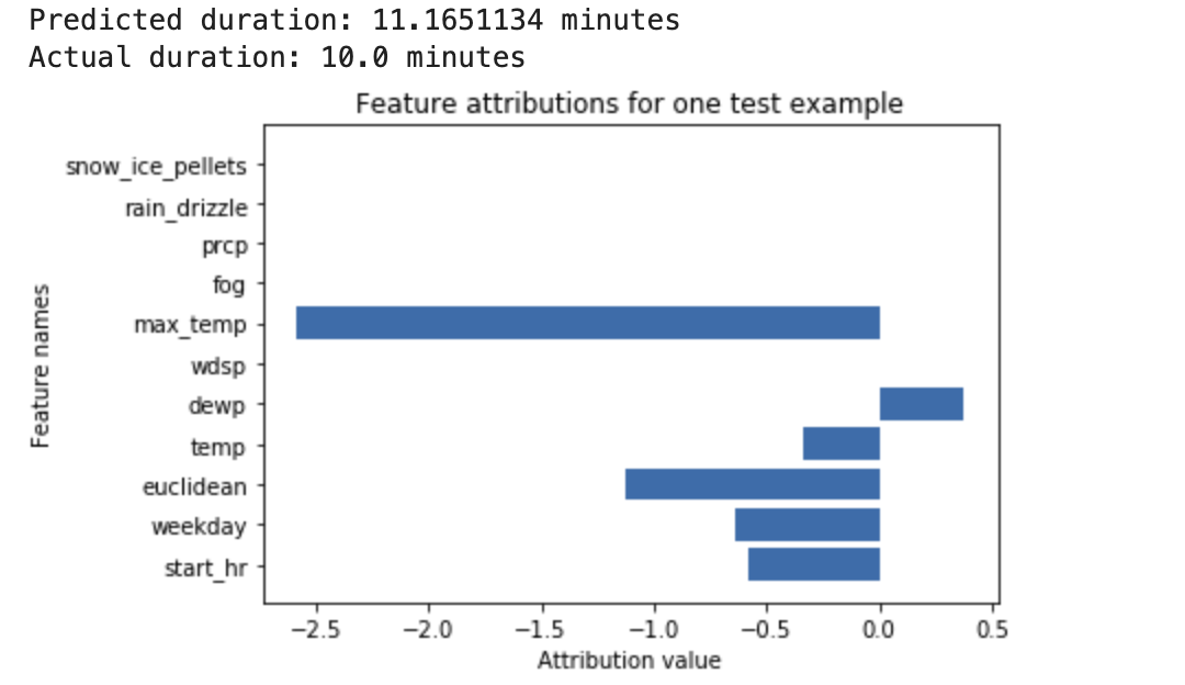
A deep neural network is trained to predict the duration of a bike ride, based on weather data and previous ride sharing data. If you request only inferences from this model, you get predicted durations of bike rides in number of minutes. If you request explanations, you get the predicted bike trip duration, along with an attribution score for each feature in your explanations request. The attribution scores show how much the feature affected the change in inference value, relative to the baseline value that you specify. Choose a meaningful baseline that makes sense for your model - in this case, the median bike ride duration. You can plot the feature attribution scores to see which features contributed most strongly to the resulting inference:

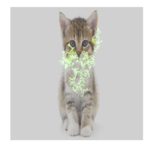
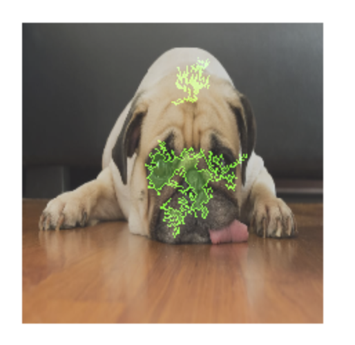
An image classification model is trained to predict whether a given image contains a dog or a cat. If you request inferences from this model on a new set of images, then you receive an inference for each image ("dog" or "cat"). If you request explanations, you get the predicted class along with an overlay for the image, showing which pixels in the image contributed most strongly to the resulting inference:

A photo of a cat with feature attribution overlay 
A photo of a dog with feature attribution overlay An image classification model is trained to predict the species of a flower in the image. If you request inferences from this model on a new set of images, then you receive an inference for each image ("daisy" or "dandelion"). If you request explanations, you get the predicted class along with an overlay for the image, showing which areas in the image contributed most strongly to the resulting inference:

A photo of a daisy with feature attribution overlay
Supported model types
Feature attribution is supported for all types of models (both AutoML and custom-trained), frameworks (TensorFlow, scikit, XGBoost), BigQuery ML models, and modalities (images, text, tabular).
To use feature attribution, configure your model for feature attribution when you upload or register the model to the Vertex AI Model Registry.
Additionally, for the following types of AutoML models, feature attribution is integrated into the Google Cloud console:
- AutoML image models (classification models only)
- AutoML tabular models (classification and regression models only)
For AutoML model types that are integrated, you can enable feature attribution in the Google Cloud console during training and see model feature importance for the model overall, and local feature importance for both online and batch inferences.
For AutoML model types that are not integrated, you can still enable feature attribution by exporting the model artifacts and configuring feature attribution when you upload the model artifacts to the Vertex AI Model Registry.
Advantages
If you inspect specific instances, and also aggregate feature attributions across your training dataset, you can get deeper insight into how your model works. Consider the following advantages:
Debugging models: Feature attributions can help detect issues in the data that standard model evaluation techniques would usually miss.
For example, an image pathology model achieved suspiciously good results on a test dataset of chest X-Ray images. Feature attributions revealed that the model's high accuracy depended on the radiologist's pen marks in the image. For more details about this example, see the AI Explanations Whitepaper.
Optimizing models: You can identify and remove features that are less important, which can result in more efficient models.
Feature attribution methods
Each feature attribution method is based on Shapley values - a cooperative game theory algorithm that assigns credit to each player in a game for a particular outcome. Applied to machine learning models, this means that each model feature is treated as a "player" in the game. Vertex Explainable AI assigns proportional credit to each feature for the outcome of a particular inference.
Sampled Shapley method
The sampled Shapley method provides a sampling approximation of exact Shapley values. AutoML tabular models use the sampled Shapley method for feature importance. Sampled Shapley works well for these models, which are meta-ensembles of trees and neural networks.
For in-depth information about how the sampled Shapley method works, read the paper Bounding the Estimation Error of Sampling-based Shapley Value Approximation.
Integrated gradients method
In the integrated gradients method, the gradient of the inference output is calculated with respect to the features of the input, along an integral path.
- The gradients are calculated at different intervals of a scaling parameter. The size of each interval is determined by using the Gaussian quadrature rule. (For image data, imagine this scaling parameter as a "slider" that is scaling all pixels of the image to black.)
- The gradients are integrated as follows:
- The integral is approximated by using a weighted average.
- The element-wise product of the averaged gradients and the original input is calculated.
For an intuitive explanation of this process as applied to images, refer to the blog post, "Attributing a deep network's inference to its input features". The authors of the original paper about integrated gradients (Axiomatic Attribution for Deep Networks) show in the preceding blog post what the images look like at each step of the process.
XRAI method
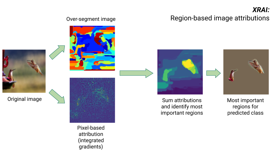
The XRAI method combines the integrated gradients method with additional steps to determine which regions of the image contribute the most to a given class inference.
- Pixel-level attribution: XRAI performs pixel-level attribution for the input image. In this step, XRAI uses the integrated gradients method with a black baseline and a white baseline.
- Oversegmentation: Independently of pixel-level attribution, XRAI oversegments the image to create a patchwork of small regions. XRAI uses Felzenswalb's graph-based method to create the image segments.
- Region selection: XRAI aggregates the pixel-level attribution within each segment to determine its attribution density. Using these values, XRAI ranks each segment and then orders the segments from most to least positive. This determines which areas of the image are most salient, or contribute most strongly to a given class inference.

Compare feature attribution methods
Vertex Explainable AI offers three methods to use for feature attributions: sampled Shapley, integrated gradients, and XRAI.
| Method | Basic explanation | Recommended model types | Example use cases | Compatible Vertex AI Model resources |
|---|---|---|---|---|
| Sampled Shapley | Assigns credit for the outcome to each feature, and considers different permutations of the features. This method provides a sampling approximation of exact Shapley values. | Non-differentiable models, such as ensembles of trees and neural networks |
|
|
| Integrated gradients | A gradients-based method to efficiently compute feature attributions with the same axiomatic properties as the Shapley value. | Differentiable models, such as neural networks. Recommended especially
for models with large feature spaces. Recommended for low-contrast images, such as X-rays. |
|
|
| XRAI (eXplanation with Ranked Area Integrals) | Based on the integrated gradients method, XRAI assesses overlapping regions of the image to create a saliency map, which highlights relevant regions of the image rather than pixels. | Models that accept image inputs. Recommended especially for natural images, which are any real-world scenes that contain multiple objects. |
|
|
For a more thorough comparison of attribution methods, see the AI Explanations Whitepaper.
Differentiable and non-differentiable models
In differentiable models, you can calculate the derivative of all the operations in your TensorFlow graph. This property helps to make backpropagation possible in such models. For example, neural networks are differentiable. To get feature attributions for differentiable models, use the integrated gradients method.
The integrated gradients method does not work for non-differentiable models. Learn more about encoding non-differentiable inputs to work with the integrated gradients method.
Non-differentiable models include non-differentiable operations in the TensorFlow graph, such as operations that perform decoding and rounding tasks. For example, a model built as an ensemble of trees and neural networks is non-differentiable. To get feature attributions for non-differentiable models, use the sampled Shapley method. Sampled Shapley also works on differentiable models, but in that case, it is more computationally expensive than necessary.
Conceptual limitations
Consider the following limitations of feature attributions:
Feature attributions, including local feature importance for AutoML, are specific to individual inferences. Inspecting the feature attributions for an individual inference may provide good insight, but the insight may not be generalizable to the entire class for that individual instance, or the entire model.
To get more generalizable insight for AutoML models, refer to the model feature importance. To get more generalizable insight for other models, aggregate attributions over subsets over your dataset, or the entire dataset.
Although feature attributions can help with model debugging, they don't always indicate clearly whether an issue arises from the model or from the data that the model is trained on. Use your best judgment, and diagnose common data issues to narrow the space of potential causes.
Feature attributions are subject to similar adversarial attacks as inferences in complex models.
For more information about limitations, refer to the high-level limitations list and the AI Explanations Whitepaper.
References
For feature attribution, the implementations of sampled Shapley, integrated gradients, and XRAI are based on the following references, respectively:
- Bounding the Estimation Error of Sampling-based Shapley Value Approximation
- Axiomatic Attribution for Deep Networks
- XRAI: Better Attributions Through Regions
Learn more about the implementation of Vertex Explainable AI by reading the AI Explanations Whitepaper.
Notebooks
To get started using Vertex Explainable AI, use these notebooks:
| Notebook | Explainability method | ML framework | Modality | Task |
|---|---|---|---|---|
| GitHub link | example-based explanations | TensorFlow | image | Train a classification model that predicts the class of the provided input image and get online explanations |
| GitHub link | feature-based | AutoML | tabular | Train a binary classification model that predicts whether a bank custom purchased a term deposit and get batch explanations |
| GitHub link | feature-based | AutoML | tabular | Train a classification model that predicts the type of Iris flower species and get online explanations |
| GitHub link | feature-based (sampled Shapley) | scikit-learn | tabular | Train a linear regression model that predicts taxi fares and get online explanations |
| GitHub link | feature-based (integrated gradients) | TensorFlow | image | Train a classification model that predicts the class of the provided input image and get batch explanations |
| GitHub link | feature-based (integrated gradients) | TensorFlow | image | Train a classification model that predicts the class of the provided input image and get online explanations |
| GitHub link | feature-based (integrated gradients) | TensorFlow | tabular | Train a regression model that predicts the median price of a house and get batch explanations |
| GitHub link | feature-based (integrated gradients) | TensorFlow | tabular | Train a regression model that predicts the median price of a house and get online explanations |
| GitHub link | feature-based (sampled Shapley) | TensorFlow | text | Train a LSTM model that classifies movie reviews as positive or negative using the text of the review and get online explanations |
Educational resources
The following resources provide further useful educational material:
- Explainable AI for Practitioners
- Interpretable Machine Learning: Shapley values
- Ankur Taly's Integrated Gradients GitHub repository.
- Introduction to Shapley values
What's next
- Configure your model for feature-based explanations
- Configure your model for example-based explanations
- View feature importance for AutoML tabular models.
