Aggregate awareness tutorial

For additional details, see the Aggregate awareness documentation page.

Introduction

This page is a guide for implementing aggregate awareness in a practical scenario, including identifying opportunities for implementation, the value aggregate awareness drives, and a simple workflow for implementing it in a real model. This page is not a deep explanation of all aggregate awareness features or edge cases, nor is it an exhaustive catalogue of all its features.

What is aggregate awareness?

In Looker, you mostly query against raw tables or views in your database. Sometimes these are Looker persistent derived tables (PDTs).

You may often encounter very large datasets or tables that, in order to be performant, require aggregation tables or roll-ups.

Commonly, you may create aggregation tables like an orders_daily table that contains limited dimensionality. These need to be treated separately and modeled separately in the Explore, and they do not sit in the model neatly. These limitations lead to poor user experiences when the user has to choose between multiple Explores for the same data.

Now, with Looker's aggregate awareness, you can pre-construct aggregate tables to various levels of granularity, dimensionality, and aggregation; and you can inform Looker of how to use them within existing Explores. Queries will then leverage these roll-up tables where Looker deems appropriate, without any user input. This will cut down query size, reduce wait times, and enhance user experience.

NOTE: Looker's aggregate tables are a type of persistent derived table (PDT). This means that aggregate tables have the same database and connection requirements as PDTs.

To see if your database dialect and Looker connection can support PDTs, see the requirements listed on the Derived tables in Looker documentation page.

To see if your database dialect supports aggregate awareness, see the Aggregate awareness documentation page.

The value of aggregate awareness

There are a number of significant value propositions aggregate awareness offers to drive extra value from your existing Looker model:

• Performance improvement: Implementing aggregate awareness will make user queries faster. Looker will use a smaller table if it contains data needed to complete the user's query.
• Cost savings: Certain dialects charge by the size of query on a consumption model. By having Looker query smaller tables, you will have a reduced cost per user query.
• User experience enhancement: Along with an improved experience that retrieves answers faster, consolidation eliminates redundant Explore creation.
• Reduced LookML footprint: Replacing existing, Liquid-based aggregate awareness strategies with flexible, native implementation leads to increased resilience and fewer errors.
• Ability to leverage existing LookML: Aggregate tables use the query object, which reuses existing modeled logic rather than duplicating logic with explicit custom SQL.

Basic example

Here is a very simple implementation in a Looker model to demonstrate how lightweight aggregate awareness can be. Given a hypothetical flights table in the database with a row for every flight recorded through the FAA, we can model this table in Looker with its own view and Explore. Here is the LookML for an aggregate table we can define for the Explore:

  explore: flights {
    aggregate_table: flights_by_week_and_carrier {
      query: {
        dimensions: [carrier, depart_week]
        measures: [cancelled_count, count]
      }

      materialization: {
        sql_trigger_value: SELECT CURRENT-DATE;;
      }
    }
  }

With this aggregate table, a user can query the flights Explore and Looker will automatically leverage the aggregate table defined above and use the aggregate table to answer queries. The user won't have to inform Looker of any special conditions, Looker will just use that table if it's a fit for the fields the user selects.

Users with see_sql permissions can use the comments in the SQL tab of an Explore to see which aggregate table will be used for a query. Here is an example Looker SQL tab for a query that uses the aggregate table flights:flights_by_week_and_carrier in teach_scratch:

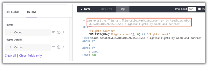
See the Aggregate awareness documentation page for details on determining if aggregate tables are used for a query.

Identifying opportunities

In order to maximize the benefits of aggregate awareness, you should identify where aggregate awareness can play a role in optimization or driving the values mentioned above.

Identify dashboards with a high runtime

One great opportunity for aggregate awareness is to create aggregate tables for heavily used dashboards with a very high runtime. You may hear from your users about slow dashboards, but if you have see_system_activity, you can also use Looker's System Activity History Explore to find dashboards with slower than average runtime. As a shortcut, you can open this System Activity History Explore link in a browser, then replace "hostname" in the URL with your Looker instance's name. You'll see an Explore visualization with data about your instance's dashboards, including Title, History, Count of Explores, Ration from Cache vs. Database, and Is Performing Worse than Mean:

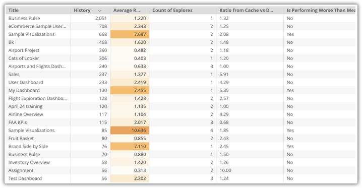
In this example, there are a number of dashboards with high utilization that perform worse than the mean, such as the Sample Visualizations dashboard. The Sample Visualizations dashboard uses two Explores, so a good strategy would be to create aggregate tables for both of these Explores.

Identify Explores that are slow and heavily queried by users

Another opportunity for aggregate awareness is with Explores that are heavily queried by users and have lower-than-average query response.

You can use the System Activity History Explore as a starting point for identifying opportunities for optimizing Explores. As a shortcut, you can open System Activity History Explore link in a browser, then replace "hostname" in the URL with your Looker instance's name. You'll see an Explore visualization with data about your instance's Explores, including Explore, Model, Query Run Count, User Count, and Average Runtime in Seconds:

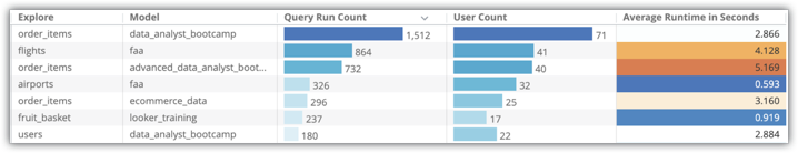
In the History Explore, you can identify the following types of Explores on your instance:

• Explores that are queried by users (as opposed to queries from the API or queries from scheduled deliveries)
• Explores that are queried often
• Explores that are performing poorly (relative to other Explores)

In the previous System Activity History Explore example, the flights and order_items Explores are probable candidates for aggregate awareness implementation.

Identify fields that are heavily used in queries

Finally, you can identify other opportunities at the data level by understanding fields that users commonly include in queries and filters.

Use the System Activity Field Usage Explore to understand the commonly selected fields within the Explores that you identified above. As a shortcut, you can open this System Activity Field Usage Explore link in a browser, then replace "hostname" in the URL with your Looker instance's name. Replace filters accordingly. You'll see an Explore with a bar graph visualization that indicates the number of times a field has been used in a query:

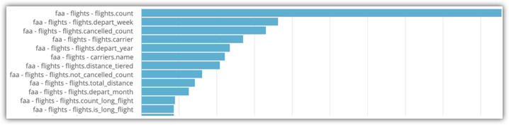
In the System Activity Explore pictured above, you can see that flights.count and flights.depart_week are the two most commonly-selected fields for the Explore. So those are good candidates for fields to include in aggregate tables.

Concrete data like this is helpful, but there are subjective elements that will guide your selection criteria. For example, by looking at the previous four fields, you can safely assume that users commonly look at the number of scheduled flights and the number of flights that were canceled and that they want to break that data down both by week and by carrier. This is an example of a clear, logical, real-world combination of fields and metrics.

Summary

The above steps should serve as a guide for finding dashboards, Explores, and fields that need to be considered for optimization. It's also worth understanding that all three may be mutually exclusive: the problematic dashboards may not be powered by the problematic Explores, and building aggregate tables with the commonly used fields may not help those dashboards at all. It is possible these are three discrete aggregate awareness implementations.

Designing aggregate tables

After you identify opportunities for aggregate awareness, you can design aggregate tables that will best address these opportunities. See the Aggregate awareness documentation page for information on the fields, measures, and timeframes supported in aggregate tables, as well as other guidelines for designing aggregate tables.

NOTE: Aggregate tables do not need to be an exact match for your query to be used. If your query is at the week granularity and you have a daily roll-up table, Looker will use your aggregate table instead of your raw, timestamp-level table. Similarly, if you have an aggregate table rolled up to the brand and date level and a user queries at the brand level only, that table is still a candidate to be used by Looker for aggregate awareness.

Aggregate awareness is supported for the following measures:

• Standard measures: Measures of type SUM, COUNT, AVERAGE, MIN, and MAX
• Composite measures: Measures of type NUMBER, STRING, YESNO, and DATE
• Approximate distinct measures: Dialects that can use HyperLogLog functionality

Aggregate awareness is not supported for the following measures:

• Distinct measures: Because distinctness can be calculated only on atomic, non-aggregated data, *_DISTINCT measures are not supported outside of these approximates that use HyperLogLog.
• Cardinality-based measures: As with distinct measures, medians and percentiles cannot be pre-aggregated and are not supported. 

NOTE: If you know of a potential user query with measure types that are not supported by aggregate awareness, this is a case where you may want to create an aggregate table that is an exact match of a query. An aggregate table that is an exact match of the query can be used to answer a query with measure types that would otherwise be unsupported for aggregate awareness.

Aggregate table granularity

Before building tables for combinations of dimensions and measures, you should determine common patterns of usage and field selection to make aggregate tables that will be used as often as possible with the biggest impact. Note that all fields used in the query (whether selected or filtered) must be in the aggregate table in order for the table to be used for the query. But, as noted previously, the aggregate table does not have to be an exact match for a query to by used for the query. You can address many potential user queries within a single aggregate table and still see large performance gains.

From the example of identifying fields that are heavily used in queries example above, there are two dimensions selected very frequently (flights.depart_week and flights.carrier), as well as two measures (flights.count and flights.cancelled_count). Therefore is would be logical to build an aggregate table that uses all four of these fields. In addition, creating a single aggregate table for flights_by_week_and_carrier will result in more frequent aggregate table usage than two different aggregate tables for flights_by_week and flights_by_carrier tables.

Here is an example aggregate table we might create for queries on the common fields:

  explore: flights {
    aggregate_table: flights_by_week_and_carrier {
      query: {
        dimensions: [carrier, depart_week]
        measures: [cancelled_count, count]
      }

      materialization: {
        sql_trigger_value: SELECT CURRENT-DATE;;
      }
    }
  }

Your business users and anecdotal evidence as well as data from Looker's System Activity can help guide your decision-making process.

Balancing applicability and performance

The following example shows an Explore query of the fields Flights Depart Week, Flights Details Carrier, Flights Count, and Flights Detailed Cancelled Count from the flights_by_week_and_carrier aggregate table:

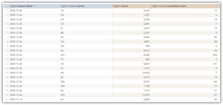
Running this query from the original database table took 15.8 seconds and scanned 38 million rows without any joins using Amazon Redshift. Pivoting the query, which would be a normal user operation, took 29.5 seconds.

After implementing the flights_by_week_and_carrier aggregate table, the subsequent query took 7.2 seconds and scanned 4592 rows . This is a 99.98% reduction in table size. Pivoting the query took 9.8 seconds.

From the System Activity Field Usage Explore, we can see how often our users include these fields in queries. In this example, flights.count was used 47,848 times, flights.depart_week was used 18,169 times, flights.cancelled_count was used 16,570 times, and flights.carrier was used 13,517 times.

Even if we very modestly estimated that 25% of these queries used all 4 fields in the simplest fashion (simple select, no pivot), 3379 x 8.6 seconds = 8 hours, 4 minutes in aggregate user wait time eliminated.

NOTE: The example model used here is very basic. These results should not be used as a benchmark or frame of reference for your model.

After applying the exact same flow to our ecommerce model order_items — the most frequently used Explore on the instance ‐ the results are as follows:

Source	Query Time	Rows Scanned
Base Table	13.1 seconds	285,000
Aggregate Table	5.1 seconds	138,000
Delta	8 seconds	147,000

The fields used in the query and subsequent aggregate table were brand, created_date, orders_count, and total_revenue, using two joins. The fields had been used a total of 11,000 times. Estimating the same combined usage of ~25%, the aggregate saving for users would be 6 hours, 6 minutes (8s * 2750 = 22000s). The aggregate table took 17.9 seconds to build.

Looking at these results, it's worth taking a moment to step back and assess the returns potentially gained from:

• Optimizing larger, more complex models/Explores that have "acceptable" performance and may see performance improvements from better modeling practices

versus

• Using aggregate awareness to optimize simpler models that are used more frequently and are performing poorly

You will see diminishing returns for your efforts as you try to get the last bit of performance from Looker and your database. You should always be cognizant of the baseline performance expectations, particularly from business users, and the limitations imposed by your database (such as concurrency, query thresholds, cost, and so on). You shouldn't expect aggregate awareness to overcome these limitations.

Also, when designing an aggregate table, remember that having more fields will result in a bigger, slower aggregate table. Bigger tables can optimize more queries and therefore be used in more situations, but large tables won't be as fast as smaller, more simple tables.

For example:

  explore: flights {
    aggregate_table: flights_by_week_and_carrier {
      query: {
        dimensions: [carrier, depart_week,flights.distance, flights.arrival_week,flights.cancelled]
        measures: [cancelled_count, count, flights.average_distance, flights.total_distance]
      }

      materialization: {
        sql_trigger_value: SELECT CURRENT-DATE;;
      }
    }
  }

This will result in the aggregate table being used for any combination of dimension shown and for any of the measures included, so this table can be used to answer many different user queries. But to use this table for a simple SELECT of carrier and count query would require a scan of an 885,000-row table. In contrast, the same query would only require a scan of 4,592 rows if the table was based on two dimensions. The 885K-row table is still a 97% reduction in table size (from the previous 38M rows); but adding one more dimension increases the table size to 20M rows. As such, there are diminishing returns as you include more fields in your aggregate table to increase its applicability to more queries.

Building aggregate tables

Taking our example Flights Explore that we identified as an opportunity to optimize, the best strategy would be to build three different aggregate tables for it:

• flights_by_week_and_carrier
• flights_by_month_and_distance
• flights_by_year

The easiest way to build these aggregate tables is to get the aggregate table LookML from an Explore query or from a dashboard and add the LookML to your Looker project files.

Once you add the aggregate tables to your LookML project and deploy the updates to production, your Explores will leverage the aggregate tables for your users' queries.

Persistence

To be accessible for aggregate awareness, aggregate tables must be persisted in your database. It is best practice to align the automatic regeneration of these aggregate tables with your caching policy by leveraging datagroups. You should use the same datagroup for an aggregate table that is used for the associated Explore. If you can't use datagroups, an alternative option is to use the sql_trigger_value parameter instead. A generic, date-based value for sql_trigger_value is shown below:

sql_trigger_value: SELECT CURRENT_DATE() ;;

This will build your aggregate tables automatically at midnight every day.

Timeframe logic

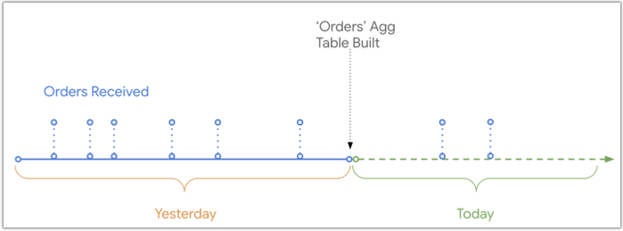
When Looker builds an aggregate table, it will include data up to the point in time the aggregate table was built. Any data that has been subsequently appended to the base table in the database would normally be excluded from the results of a query using that aggregate table.

This diagram shows the timeline of when orders were received and logged in the database compared to the the point in time that the Orders aggregate table was built. There are two orders received today that will not be present in the Orders aggregate table, since the orders were received after the aggregate table was built:

But Looker can UNION fresh data to the aggregate table when a user queries for a timeframe that overlaps with the aggregate table, as depicted in the same timeline diagram:

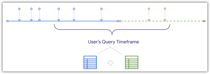
Because Looker can UNION fresh data to an aggregate table, if a user filters for a timeframe that overlaps with the end of both the aggregate and the base table, the orders received after the aggregate table was built will be included in the user's results. See the Aggregate awareness documentation page for details and the conditions that need to be met to union fresh data to aggregate table queries.

Summary

To recap, to build an aggregate awareness implementation, there are three fundamental steps:

1. Identify opportunities where optimization using aggregate tables is appropriate and impactful.
2. Design aggregate tables that will provide the most coverage for common user queries while still remaining small enough to reduce the size of those queries sufficiently.
3. Build the aggregate tables in the Looker model, pairing the persistence of the table with the persistence of the Explore cache.