This tutorial introduces you to geospatial analytics. Geospatial analytics lets you analyze and visualize geospatial data in BigQuery.
Objectives
In this tutorial, you:
- Use a geospatial analytics function to convert latitude and longitude columns into geographical points
- Run a query that finds all the Citi Bike stations with more than 30 bikes available for rental
- Visualize your results in BigQuery
- Visualize your results in BigQuery Geo Viz
Costs
This tutorial uses billable components of Google Cloud, including BigQuery.
You incur charges for:
- Querying data in the
BigQuery public datasets.
- The first 1 TB is free each month.
- If you are using capacity-based pricing, query costs are included in the capacity-based price.
Before you begin
- Sign in to your Google Cloud account. If you're new to Google Cloud, create an account to evaluate how our products perform in real-world scenarios. New customers also get $300 in free credits to run, test, and deploy workloads.
-
In the Google Cloud console, on the project selector page, select or create a Google Cloud project.
Roles required to select or create a project
- Select a project: Selecting a project doesn't require a specific IAM role—you can select any project that you've been granted a role on.
-
Create a project: To create a project, you need the Project Creator
(
roles/resourcemanager.projectCreator), which contains theresourcemanager.projects.createpermission. Learn how to grant roles.
-
Verify that billing is enabled for your Google Cloud project.
-
In the Google Cloud console, on the project selector page, select or create a Google Cloud project.
Roles required to select or create a project
- Select a project: Selecting a project doesn't require a specific IAM role—you can select any project that you've been granted a role on.
-
Create a project: To create a project, you need the Project Creator
(
roles/resourcemanager.projectCreator), which contains theresourcemanager.projects.createpermission. Learn how to grant roles.
-
Verify that billing is enabled for your Google Cloud project.
- BigQuery is automatically enabled in new projects.
To activate BigQuery in an existing project, go to
Enable the BigQuery API.
Roles required to enable APIs
To enable APIs, you need the Service Usage Admin IAM role (
roles/serviceusage.serviceUsageAdmin), which contains theserviceusage.services.enablepermission. Learn how to grant roles.
Explore the sample data
This tutorial uses a dataset available through the Google Cloud Public Dataset Program. A public dataset is any dataset that is stored in BigQuery and made available to the general public. The public datasets are datasets that BigQuery hosts for you to access and integrate into your applications. Google pays for the storage of these datasets and provides public access to the data by using a project. You pay only for the queries that you perform on the data (the first 1 TB per month is free, subject to query pricing details.)
The NYC Citi Bike Trips dataset
Citi Bike is the nation's largest bike share program, with 10,000 bikes and 600 stations across Manhattan, Brooklyn, Queens, and Jersey City. This dataset includes Citi Bike trips since Citi Bike launched in September 2013 and is updated daily. The data is processed by Citi Bike to remove trips that are taken by staff to service and inspect the system and any trips that are less than 60 seconds in duration, which are considered false starts.
You can start exploring this data in the BigQuery console by
viewing the details of the citibike_stations table:
Go to citibike_stations schema
Three columns in this table are relevant to this tutorial:
bike_stations.longitude: the longitude of a station. The values are valid WGS 84 longitudes in decimal degrees format.bike_stations.latitude: the latitude of a station. The values are valid WGS 84 latitudes in decimal degrees format.num_bikes_available: the number of bikes available for rental.
Query the bike stations with more than 30 bikes available
In this section of the tutorial, you run a GoogleSQL query that finds all the Citi Bike stations in New York City with more than 30 bikes available to rent.
Query details
The following GoogleSQL query is used to find the Citi Bike stations with more than 30 bikes.
SELECT
  ST_GeogPoint(longitude, latitude)  AS WKT,
  num_bikes_available
FROM
  `bigquery-public-data.new_york.citibike_stations`
WHERE num_bikes_available > 30
The query clauses do the following:
SELECT ST_GeogPoint(longitude, latitude) AS WKT, num_bikes_available- The
SELECTclause selects thenum_bikes_availablecolumn and uses theST_GeogPointfunction to convert the values in thelatitudeandlongitudecolumns toGEOGRAPHYtypes (points).
FROM `bigquery-public-data.new_york.citibike_stations`- The
FROMclause specifies the table being queried:citibike_stations.
WHERE num_bikes_available > 30- The
WHEREclause filters the values in thenum_bikes_availablecolumn to just those stations with more than 30 bikes.
Run the query
To run the query by using the Google Cloud console:
Go to the BigQuery page in the Google Cloud console.
Enter the following GoogleSQL query in the Query editor text area.
-- Finds Citi Bike stations with > 30 bikes
SELECT
  ST_GeogPoint(longitude, latitude)  AS WKT,
  num_bikes_available
FROM
  `bigquery-public-data.new_york.citibike_stations`
WHERE num_bikes_available > 30
Click Run.
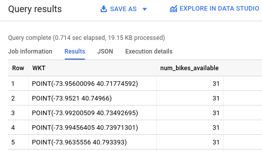
The query takes a moment to complete. After the query runs, your results appear in the Query results pane.
Visualize the results in BigQuery
To visualize the results in an interactive map, follow these steps:
In the Query results pane, click Visualization.
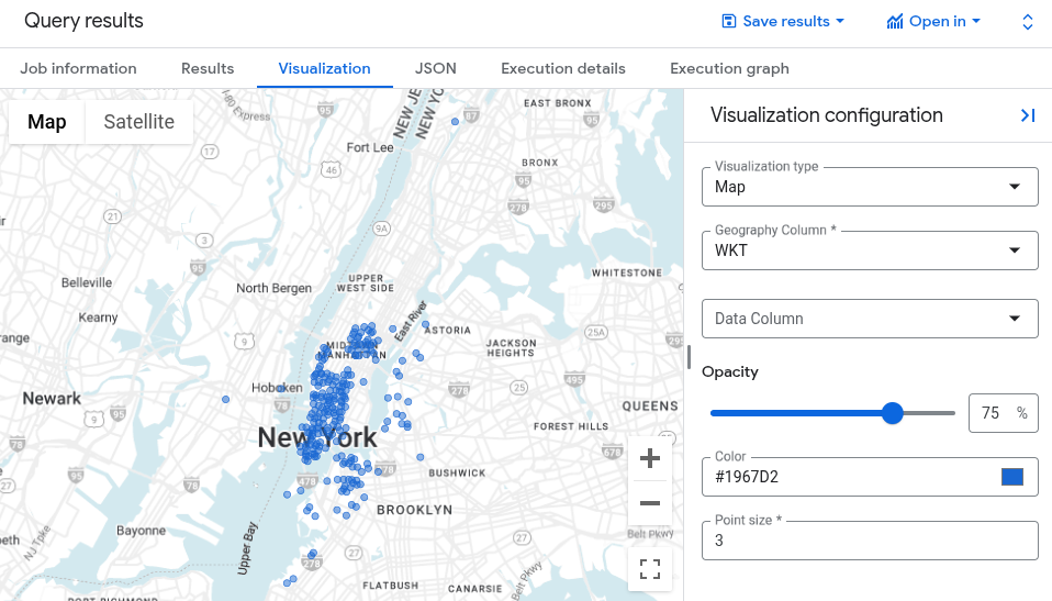
The points on the map show the locations of each bike station.
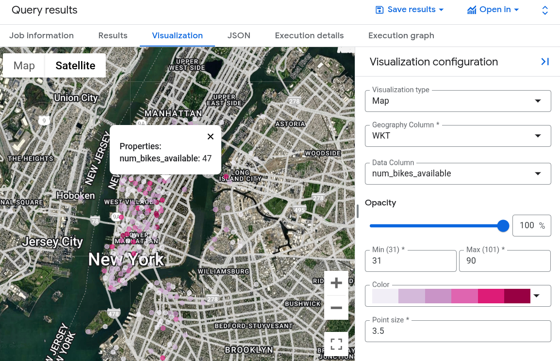
You can apply uniform or data driven styling to your map. To visualize how many bikes are available at each station, for Data column select
num_bikes_available.To improve visibility, try adjusting the Opacity, Color, or Point size. If your data contains outliers, you can adjust the Min and Max values. Geographies with values outside this range are still displayed on the map, but no color is applied.
To view the properties of a geography, click it.
To view the map in satellite mode, click Satellite.
Visualize the query results in Geo Viz
You can also visualize your results using BigQuery Geo Viz: a web tool for visualization of geospatial data in BigQuery using Google Maps APIs.
Launch Geo Viz and authenticate
Before using Geo Viz, you must authenticate and grant access to data in BigQuery.
To set up Geo Viz:
Open the Geo Viz web tool.
You might need to enable cookies to authorize and use this tool.
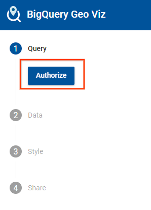
Under step one, Query, click Authorize.
In the Choose an account dialog, click your Google Account.

In the access dialog, click Allow to give Geo Viz access to your BigQuery data.

Run a GoogleSQL query on geospatial data
After you authenticate and grant access, the next step is to run the query in Geo Viz.
To run the query:
For step one, Select data, enter your project ID in the Project ID field.
In the query window, enter the following GoogleSQL query.
-- Finds Citi Bike stations with > 30 bikes
SELECT
  ST_GeogPoint(longitude, latitude)  AS WKT,
  num_bikes_available
FROM
  `bigquery-public-data.new_york.citibike_stations`
WHERE num_bikes_available > 30
Click Run.
When the query completes, click Show results. You can also click step two Define columns.
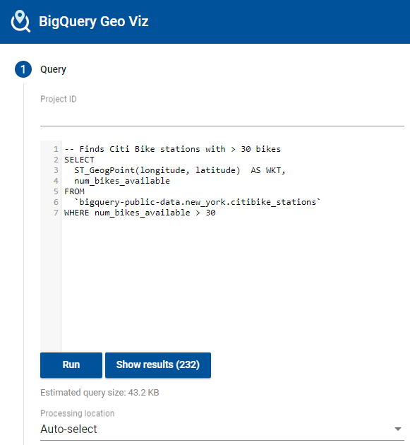
This moves you to step two. In step two, for Geometry column, choose WKT. This plots the points corresponding to the bike stations on your map.
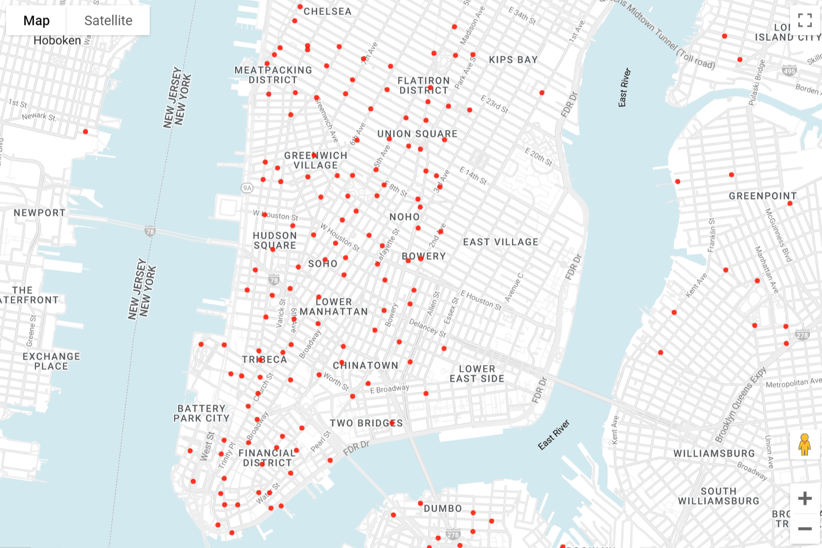
Format your visualization
The Style section provides a list of visual styles for customization. Certain
properties apply only to certain types of data. For example, circleRadius
affects only points.
Supported style properties include:
- fillColor. The fill color of a polygon or point. For example, "linear" or "interval" functions can be used to map numeric values to a color gradient.
- fillOpacity. The fill opacity of a polygon or point. Values must be
in the range 0 to 1, where
0= transparent and1= opaque. - strokeColor. The stroke or outline color of a polygon or line.
- strokeOpacity. The stroke or outline opacity of polygon or line.
Values must be in the range 0 to 1, where
0= transparent and1= opaque. - strokeWeight. The stroke or outline width in pixels of a polygon or line.
- circleRadius. The radius of the circle representing a point in pixels. For example, a "linear" function can be used to map numeric values to point sizes to create a scatterplot style.
Each style can be given either a global value (applied to every result) or a data-driven value (applied in different ways depending on data in each result row). For data-driven values, the following are used to determine the result:
- function. A function used to compute a style value from a field's values.
- identity. The data value of each field is used as the styling value.
- categorical. The data values of each field listed in the domain are mapped one to one with corresponding styles in the range.
- interval. Data values of each field are rounded down to the nearest value in the domain and are then styled with the corresponding style in the range.
- linear. Data values of each field are interpolated linearly across values in the domain and are then styled with a blend of the corresponding styles in the range.
- field. The specified field in the data is used as the input to the styling function.
- domain. An ordered list of sample input values from a field. Sample inputs (domain) are paired with sample outputs (range) based on the given function and are used to infer style values for all inputs (even those not listed in the domain). Values in the domain must have the same type (text, number, and so on) as the values of the field you are visualizing.
- range. A list of sample output values for the style rule. Values in
the range must have the same type (color or number) as the style property you
are controlling. For example, the range of the
fillColorproperty should contain only colors.
To format your map:
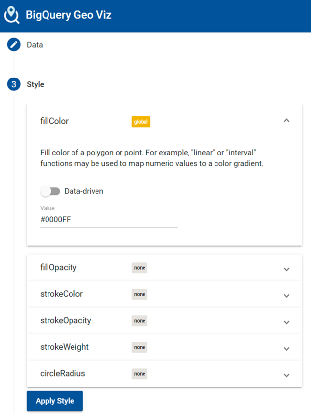
Click Add styles in step two or click step 3 Style.
Change the color of your points. Click fillColor.
In the Value field, enter
#0000FF, the HTML color code for blue.Click Apply Style.
Examine your map. If you click one of your points, the value is displayed.
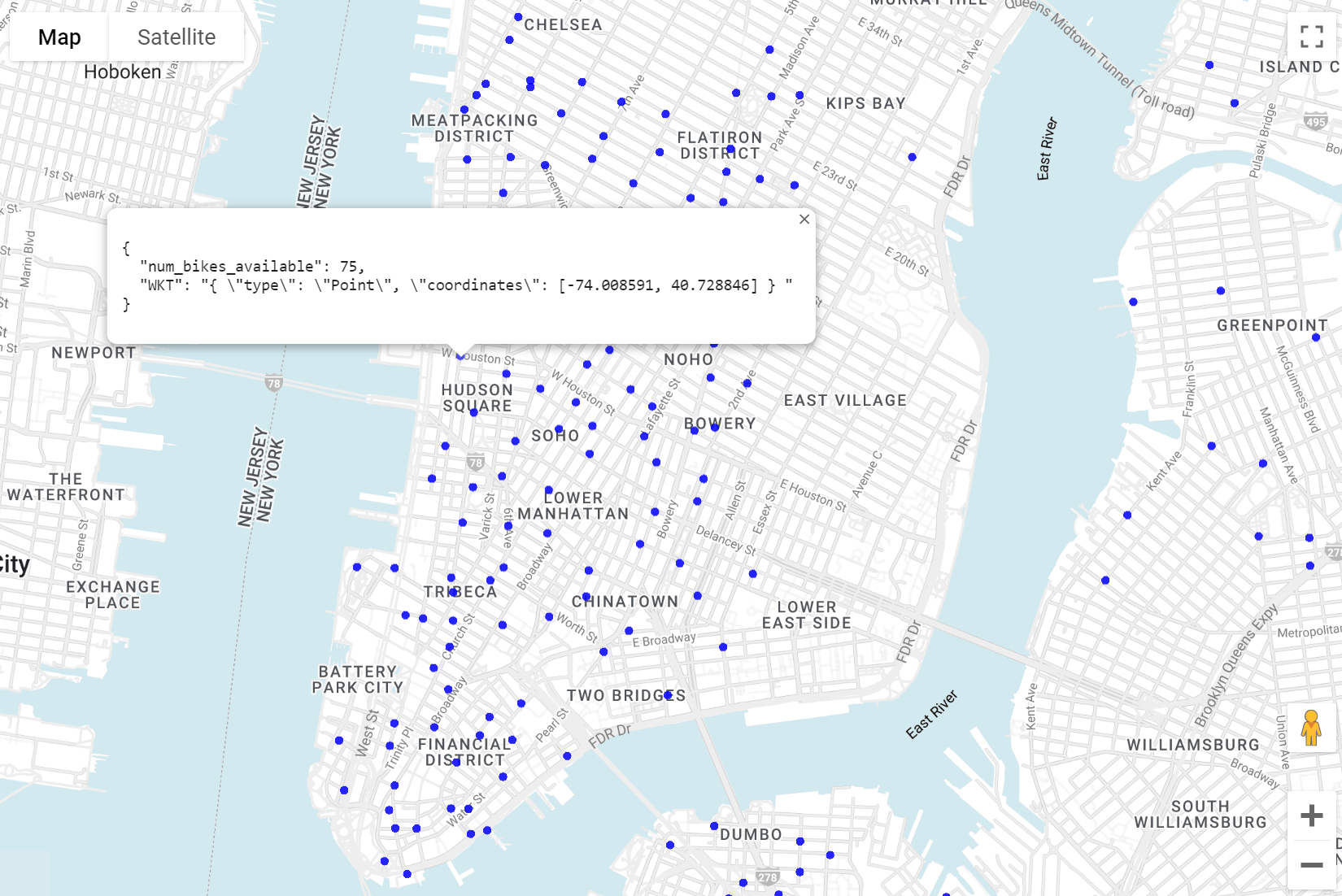
Click fillOpacity.
In the Value field, enter
0.5and click Apply Style.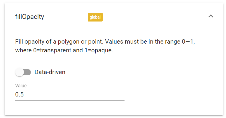
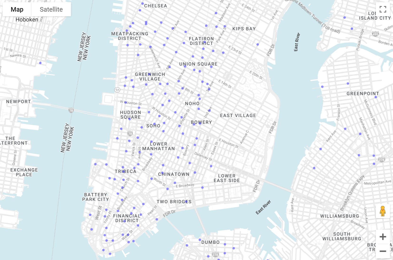
Examine your map. The fill color of the points is now semi-transparent.
Change the size of the points based on the number of bikes available. Click circleRadius.
In the circleRadius panel:
- Click Data driven.
- For Function, choose linear.
- For Field, choose
num_bikes_available. - For Domain, enter
30in the first box and60in the second. For Range, enter
5in the first box and20in the second.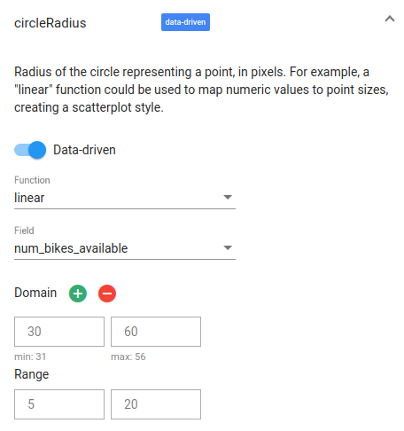
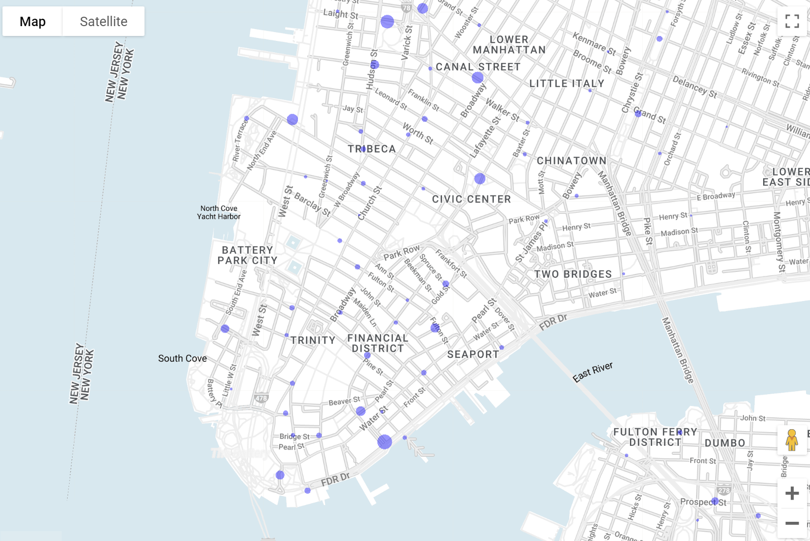
Examine your map. The radius of each circle now corresponds to the number of bikes available at that location.
Close Geo Viz.
Clean up
To avoid incurring charges to your Google Cloud account for the resources used in this tutorial, either delete the project that contains the resources, or keep the project and delete the individual resources.
- You can delete the project you created.
- Or you can keep the project for future use.
To delete the project:
- In the Google Cloud console, go to the Manage resources page.
- In the project list, select the project that you want to delete, and then click Delete.
- In the dialog, type the project ID, and then click Shut down to delete the project.
What's next
- To learn more about visualization options for geospatial analytics, see Visualizing geospatial data.
- To learn more about working with geospatial analytics data, see Working with geospatial data.
- For a tutorial on using geospatial analytics, see Using geospatial analytics to plot a hurricane's path.
- For documentation on GoogleSQL functions in geospatial analytics, see Geography functions in GoogleSQL.
