Migrate from DynamoDB to Bigtable
Bigtable and DynamoDB are distributed key-value stores that can support millions of queries per second (QPS), provide storage that scales up to petabytes of data, and tolerate node failures.
This document is intended for DynamoDB developers and database administrators who want to migrate to Bigtable. It's also useful when you want to design applications for use with Bigtable as a datastore.
To get started, use a Google-provided migration tool that helps you migrate from DynamoDB to Bigtable. This page describes the migration tool, compares the two database systems, and describes the underlying architecture and interaction details that differ and that are important to understand before migrating.
Get started with the DynamoDB-to-Bigtable migration tool
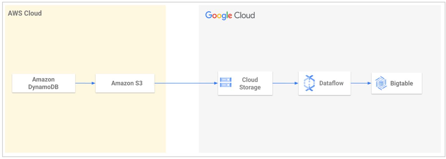
An open source migration tool is provided by Google Cloud Professional Services to streamline the migration of data from DynamoDB to Bigtable. The tool automates the process of importing your data to Google Cloud and then loading it into Bigtable.
Using the tool, you export your DynamoDB table and then transfer it to Cloud Storage. The tool reads the exported files from your Cloud Storage bucket and uses a Dataflow template to transform the data so that it's compatible with Bigtable. This transformation includes mapping DynamoDB attributes to Bigtable rows. The Dataflow job then writes the transformed data to your Bigtable table.
For more information or to get started, see DynamoDB to Bigtable Migration Utility.
Comparison of DynamoDB and Bigtable
This section examines the similarities and differences between DynamoDB and Bigtable.
Control plane
In DynamoDB and Bigtable, the control plane lets you configure your capacity and set up and manage resources. DynamoDB is a serverless product, and the highest level of interaction with DynamoDB is the table level. In provisioned capacity mode, this is where you provision your read and write request units, select your regions and replication, and manage backups. Bigtable is not a serverless product; you must create an instance with one or more clusters, whose capacity is determined by the number of nodes that they have. For details on these resources, see Instances, clusters, and nodes.
The following table compares control plane resources for DynamoDB and Bigtable.
| DynamoDB | Bigtable |
|---|---|
| Table: A collection of items with a defined primary key. Tables have settings for backups, replication, and capacity. | Instance: A group of Bigtable clusters
in different Google Cloud zones or regions, between which replication
and connection routing occur. Replication policies are set at the
instance level. Cluster: A group of nodes in the same geographic Google Cloud zone, ideally colocated with your application server for latency and replication reasons. Capacity is managed by adjusting the number of nodes in each cluster. Table: A logical organization of values that's indexed by row key. Backups are controlled at the table level. |
Read capacity unit (RCU) and write capacity unit (WCU):
Units allowing for reads or writes per second with fixed
payload size. You are charged for read or write units for each
operation with larger payload sizes.UpdateItem operations consume the write capacity used for the
largest size of an updated item – either before or after the update –
even if the update involves a subset of the item's attributes. |
Node: A virtual compute resource responsible for
reading and writing data. The number of nodes that a cluster has
translates to throughput limits for reads, writes, and scans. You can
adjust the number of nodes, depending on the combination of your
latency goals, request count, and payload size. SSD nodes deliver the same throughput for reads and writes, unlike the significant difference between RCU and WCU. For more information, see Performance for typical workloads. |
| Partition: A block of contiguous rows, backed by
solid state drives (SSDs) colocated with nodes. Each partition is subject to a hard limit of 1,000 WCUs, 3,000 RCUs, and 10 GB of data. |
Tablet: A block of contiguous rows backed by the
storage medium of choice (SSD or HDD). Tables are sharded into tablets to balance the workload. Tablets are not stored on nodes in Bigtable but rather on Google's distributed file system, which allows speedy redistribution of data when scaling, and which provides additional durability by maintaining multiple copies. |
| Global tables: A way to increase availability and durability of your data by automatically propagating data changes across multiple regions. | Replication: A way to increase the availability and durability of your data by automatically propagating data changes across multiple regions or multiple zones within the same region. |
| Not applicable (N/A) | Application profile: Settings that instruct Bigtable how to route a client API call to the appropriate cluster in the instance. You can also use an app profile as a tag to segment metrics for attribution. |
Geographic replication
Replication is used to support customer requirements for the following:
- High availability for business continuity in the event of a zonal or regional failure.
- Putting your service data in close proximity to end users for low-latency serving wherever they are in the world.
- Workload isolation when you need to implement a batch workload on one cluster and rely on replication to serving clusters.
Bigtable supports replicated clusters in as many zones that are available in up to 8 Google Cloud regions where Bigtable is available. Most regions have three zones. For more information, see Regions and zones.
Bigtable automatically replicates data across clusters in a multi-primary topology, meaning you can read and write to any cluster. Bigtables replication is eventually consistent. For details, see the Replication overview.
DynamoDB provides global tables to support table replication across multiple regions. Global tables are multi-primary and replicate automatically across regions. Replication is eventually consistent.
The following table lists replication concepts and describes their availability in DynamoDB and Bigtable.
| Property | DynamoDB | Bigtable |
|---|---|---|
| Multi-primary replication | Yes. You can read and write to any global table. |
Yes. You can read and write to any Bigtable cluster. |
| Consistency model | Eventually consistent. Read-your-writes consistency at the regional level for global tables. |
Eventually consistent. Read-your-writes consistency at the cluster level for all tables provided that you send both reads and writes to the same cluster. |
| Replication latency | No service level agreement (SLA). Seconds |
No SLA. Seconds |
| Configuration granularity | Table level. | Instance level. An instance can contain multiple tables. |
| Implementation | Create a global table with a table replica in each selected
region. Regional level. Automatic replication across replicas by converting a table to a global table. The tables must have DynamoDB Streams enabled, with the stream containing both the new and the old images of the item. Delete a region to remove the global table in that region. |
Create an instance with more than one cluster. Replication is automatic across clusters in that instance. Zonal level. Add and remove clusters from a Bigtable instance. |
| Replication options | Per table. | Per instance. |
| Traffic routing and availability | Traffic routed to the nearest geographical replica. In the event of failure, you apply custom business logic to determine when to redirect requests to other regions. |
Use application profiles to configure
cluster traffic routing policies. Use multi-cluster routing to route traffic automatically to the nearest healthy cluster. In the event of failure, Bigtable supports automatic failover between clusters for HA. |
| Scaling | Write capacity in replicated write request units (R-WRU) is
synchronized across replicas. Read capacity in replicated read capacity units (R-RCU) is per replica. |
You can scale clusters independently by adding or removing nodes from each replicated cluster as required. |
| Cost | R-WRUs cost 50% more than regular WRUs. | You are billed for each cluster's nodes and storage. There are no network replication costs for regional replication across zones. Costs are incurred when replication is across regions or continents. |
| SLA | 99.999% | 99.999% |
Data plane
The following table compares data model concepts for DynamoDB and Bigtable. Each row in the table describes analogous features. For example, an item in DynamoDB is similar to a row in Bigtable.
| DynamoDB | Bigtable |
|---|---|
| Item: A group of attributes that is uniquely identifiable among all of the other items by its primary key. Maximum allowed size is 400 KB. | Row: A single entity identified by the row key. Maximum allowed size is 256 MB. |
| N/A | Column family: A user-specified namespace that groups columns. |
| Attribute: A grouping of a name and a value. An attribute value can be a scalar, set, or document type. There is no explicit limit on attribute size itself. However, because each item is limited to 400 KB, for an item that only has one attribute, the attribute can be up to 400 KB minus the size occupied by the attribute name. | Column qualifier: The unique identifier within a
column family for a column. The full identifier of a column is
expressed as column-family:column-qualifier. Column qualifiers are
lexicographically sorted within the column family. The maximum allowed size for a column qualifier is 16 KB. Cell: A cell holds the data for a given row, column, and timestamp. A cell contains one value that can be up to 100 MB. |
| Primary key: A unique identifier for an item in a
table. It can be a partition key or a composite key. Partition key: A simple primary key, composed of one attribute. This determines the physical partition where the item is located. Maximum allowed size is 2 KB. Sort key: A key that determines the ordering of rows within a partition. Maximum allowed size is 1 KB. Composite key: A primary key composed of two properties, the partition key and a sort key or range attribute. |
Row key: A unique identifier for an item in a table.
Typically represented by a concatenation of values and delimiters.
Maximum allowed size is 4 KB. Column qualifiers can be used to deliver behavior equivalent to that of DynamoDB's sort key. Composite keys can be built using concatenated row keys and column qualifiers. For more details, see the schema translation example in the Schema design section of this document. |
| Time to live: Per-item timestamps determine when an item is no longer needed. After the date and time of the specified timestamp, the item is deleted from your table without consuming any write throughput. | Garbage collection: Per-cell timestamps determine when an item is no longer needed. Garbage collection deletes expired items during a background process called compaction. Garbage collection policies are set at the column family level and can delete items not only based on their age but also according to the number of versions the user wants to maintain. You don't need to accommodate capacity for compaction while sizing your clusters. |
| Global secondary index: A table that contains selected attributes from the base table, organized by a primary key that is different from that of the table. The index key doesn't need to include any of the key attributes from the table. It doesn't need to have the same key schema as the table. DynamoDB updates global secondary indexes asynchronously. | Asynchronous secondary index: To query the same data using different lookup patterns or attributes, you can create an asynchronous secondary index. This type of index contains selected attributes from the base table. These attributes are organized by a key that is different from the table's own key. The behavior is similar to DynamoDB global secondary indexes. |
Operations
Data plane operations let you perform create, read, update, and delete (CRUD) actions on data in a table. The following table compares similar data plane operations for DynamoDB and Bigtable.
| DynamoDB | Bigtable |
|---|---|
CreateTable |
CreateTable |
PutItemBatchWriteItem |
MutateRow MutateRowsBigtable treats write operations as upserts. |
UpdateItem
|
Bigtable treats write operations as upserts. |
GetItemBatchGetItem, Query, Scan |
`ReadRow`` ReadRows` (range, prefix, reverse scan)Bigtable supports efficient scanning by row key prefix, regular expression pattern, or row key range forward or backward. |
Data types
Both Bigtable and DynamoDB are schemaless. Columns can be defined at write-time without any table-wide enforcement for column existence or data types. Similarly, a given column or attribute data type can differ from one row or item to another. However, the DynamoDB and Bigtable APIs deal with data types in different ways.
Each DynamoDB write request includes a type definition for each attribute, which is returned with the response for read requests.
Bigtable treats everything as bytes and expects the client code to know the type and encoding so the client can parse the responses correctly. An exception is increment operations, which interpret the values as 64-bit big-endian signed integers.
The following table compares the differences in data types between DynamoDB and Bigtable.
| DynamoDB | Bigtable |
|---|---|
| Scalar types: Returned as data type descriptor tokens in the server response. | Bytes: Bytes are cast to intended types in the client
application. Increment interprets the value as 64-bit big-endian signed integer |
| Set: An unsorted collection of unique elements. | Column family: You can use column qualifiers as set member names and for each one, provide a single 0 byte as the cell value. Set members are sorted lexicographically within their column family. |
| Map: An unsorted collection of key-value pairs with unique keys. | Column family Use column qualifier as map key and cell value for value. Map keys are sorted lexicographically. |
| List: A sorted collection of items. | Column qualifier Use the insert timestamp to achieve the equivalent of list_append behavior, reverse of insert timestamp for prepend. |
Schema design
An important consideration in schema design is how the data is stored. Among the key differences between Bigtable and DynamoDB are how they handle the following:
- Updates to single values
- Data sorting
- Data versioning
- Storage of large values
Updates to single values
UpdateItem operations in DynamoDB consume the write capacity for the larger of
the "before" and "after" item sizes even if the update involves a subset of the
item's attributes. This means that in DynamoDB, you might put frequently updated
columns in separate rows, even if logically they belong in the same row with
other columns.
Bigtable can update a cell just as efficiently whether it is the only column in a given row or one among many thousands. For details, see Simple writes.
Data sorting
DynamoDB hashes and randomly distributes partition keys, whereas Bigtable stores rows in lexicographical order by row key and leaves any hashing up to the user.
Random key distribution isn't optimal for all access patterns. It reduces the risk of hot row ranges, but it makes access patterns that involve scans that cross partition boundaries expensive and inefficient. These unbounded scans are common, especially for use cases that have a time dimension.
Handling this type of access pattern — scans that cross partition boundaries — requires a secondary index in DynamoDB, but not in Bigtable. While you can design the lexicographical row key in Bigtable to handle many scan patterns efficiently, Bigtable also supports asynchronous secondary indexes that you implement as continuous materialized views to provide efficient, eventually consistent lookups for alternative query patterns. Similarly, in DynamoDB, query and scan operations are limited to 1 MB of data scanned, which requires pagination beyond this limit. Bigtable has no such limit.
Despite its randomly distributed partition keys, DynamoDB can still have hot partitions if a chosen partition key doesn't uniformly distribute traffic that is adversely affecting throughput. To address this issue, DynamoDB advises write-sharding, randomly splitting writes across multiple logical partition key values.
To apply this design pattern, you need to create a random number from a fixed set (for example, 1 to 10), and then use this number as the logical partition key. Because you are randomizing the partition key, the writes to the table are spread evenly across all of the partition key values.
Bigtable refers to this procedure as key salting, and it can be an effective way to avoid hot tablets.
Data versioning
Each Bigtable cell has a timestamp, and the most recent timestamp is always the default value for any given column. A common use case for timestamps is versioning — writing a new cell to a column that is differentiated from previous versions of the data for that row and column by its timestamp.
DynamoDB doesn't have such a concept and requires
complex schema designs
to support versioning. This approach involves creating two copies of each item:
one copy with a version-number prefix of zero, such as v0_, at the beginning
of the sort key, and another copy with a version-number prefix of one, such as
v1_. Every time the item is updated, you use the next higher version-prefix in
the sort key of the updated version, and copy the updated contents into the item
with version-prefix zero. This ensures that the latest version of any item can
be located using the zero prefix. This strategy not only requires
application side logic to maintain but also makes data writes very expensive and
slow, because each write requires a read of the previous value plus two
writes.
Multi-row transactions versus large row capacity
Bigtable doesn't support multi-row transactions. However, because it lets you store rows that are much larger than items can be in DynamoDB, you can often get the intended transactionality by designing your schemas to group relevant items under a shared row key. For an example that illustrates this approach, see Single table design pattern.
Storing large values
Since a DynamoDB item, which is analogous to a Bigtable row, is limited to 400 KB, storing large values requires either splitting the value across items or storing in other media like S3. Both of these approaches add complexity to your application. In contrast, a Bigtable cell can store up to 100 MB, and a Bigtable row can support up to 256 MB.
Schema translation examples
The examples in this section translate schemas from DynamoDB to Bigtable with the key schema design differences in mind.
Migrating basic schemas
Product catalogs are a good example to demonstrate the basic key-value pattern. The following is what such a schema might look like in DynamoDB.
| Primary Key | Attributes | |||
|---|---|---|---|---|
| Partition key | Sort key | Description | Price | Thumbnail |
| hats | fedoras#brandA | Crafted from premium wool… | 30 | https://storage… |
| hats | fedoras#brandB | Durable water-resistant canvas built to.. | 28 | https://storage… |
| hats | newsboy#brandB | Add a touch of vintage charm to your everyday look.. | 25 | https://storage… |
| shoes | sneakers#brandA | Step out in style and comfort with… | 40 | https://storage… |
| shoes | sneakers#brandB | Classic features with contemporary materials… | 50 | https://storage… |
For this table, mapping from DynamoDB to Bigtable is straightforward: you convert DynamoDB's composite primary key into a composite Bigtable row key. You create one column family (SKU) that contains the same set of columns.
| SKU | |||
|---|---|---|---|
| Row key | Description | Price | Thumbnail |
| hats#fedoras#brandA | Crafted from premium wool… | 30 | https://storage… |
| hats#fedoras#brandB | Durable water-resistant canvas built to.. | 28 | https://storage… |
| hats#newsboy#brandB | Add a touch of vintage charm to your everyday look.. | 25 | https://storage… |
| shoes#sneakers#brandA | Step out in style and comfort with… | 40 | https://storage… |
| shoes#sneakers#brandB | Classic features with contemporary materials… | 50 | https://storage… |
Single table design pattern
A single table design pattern brings together what would be multiple tables in a relational database into a single table in DynamoDB. You can take the approach in the previous example and duplicate this schema as-is in Bigtable. However, it's better to address the schema's problems in the process.
In this schema, the partition key contains the unique ID for a video, which
helps colocate all attributes related to that video for faster access. Given
DynamoDB's item size limitations, you can't put an unlimited number of free text
comments in a single row. Therefore, a sort key with the pattern
VideoComment#reverse-timestamp is used to make each comment a separate row
within the partition, sorted in reverse chronological order.
Assume this video has 500 comments and the owner wants to remove the video. This means that all the comments and video attributes also need to be deleted. To do this in DynamoDB, you need to scan all the keys within this partition and then issue multiple delete requests, iterating through each. DynamoDB supports multi-row transactions, but this delete request is too large to do in a single transaction.
| Primary Key | Attributes | |||
|---|---|---|---|---|
| Partition key | Sort key | UploadDate | Formats | |
| 0123 | Video | 2023-09-10T15:21:48 | {"480": "https://storage…", "720": "https://storage…", "1080p": "https://storage…"} | |
| VideoComment#98765481 | Content | |||
| I really like this. Special effects are amazing. | ||||
| VideoComment#86751345 | Content | |||
| There seems to be an audio glitch at 1:05. | ||||
| VideoStatsLikes | Count | |||
| 3 | ||||
| VideoStatsViews | Count | |||
| 156 | ||||
| 0124 | Video | 2023-09-10T17:03:21 | {"480": "https://storage…", "720": "https://storage…"} | |
| VideoComment#97531849 | Content | |||
| I shared this with all my friends. | ||||
| VideoComment#87616471 | Content | |||
| The style reminds me of a movie director but I can't put my finger on it. | ||||
| VideoStats | ViewCount | |||
| 45 | ||||
Modify this schema as you migrate so that you can simplify your code and make data requests faster and cheaper. Bigtable rows have much larger capacity than DynamoDB items and can handle a large number of comments. To handle a case where a video gets millions of comments, you can set a garbage collection policy to only keep a fixed number of most recent comments.
Because counters can be updated without the overhead of updating the entire row, you don't have to split them, either. You don't have to use an UploadDate column or calculate a reverse timestamp and make that your sort key, either, because Bigtable timestamps give you the reverse chronologically ordered comments automatically. This significantly simplifies the schema, and if a video is removed, you can transactionally remove the video's row, including all the comments, in a single request.
Lastly, because columns in Bigtable are ordered lexicographically, as an optimization, you can rename the columns in a way that allows a fast range scan – from video properties to the top N most recent comments – in a single read request, which is what you'd want to do when the video is loaded. Then later, you can page through the rest of the comments as the viewer scrolls.
| Attributes | ||||
|---|---|---|---|---|
| Row key | Formats | Likes | Views | UserComments |
| 0123 | {"480": "https://storage…", "720": "https://storage…", "1080p": "https://storage…"} @2023-09-10T15:21:48 | 3 | 156 | I really like this. Special effects are amazing. @
2023-09-10T19:01:15 There seems to be an audio glitch at 1:05. @ 2023-09-10T16:30:42 |
| 0124 | {"480": "https://storage…", "720":"https://storage…"} @2023-09-10T17:03:21 | 45 | The style reminds me of a movie director but I can't put my finger on it. @2023-10-12T07:08:51 | |
Adjacency list design pattern
Consider a slightly different version of this design, which DynamoDB often refers to as the adjacency list design pattern.
| Primary Key | Attributes | |||
|---|---|---|---|---|
| Partition key | Sort key | DateCreated | Details | |
| Invoice-0123 | Invoice-0123 | 2023-09-10T15:21:48 | {"discount": 0.10, "sales_tax_usd":"8", "due_date":"2023-10-03.."} |
|
| Payment-0680 | 2023-09-10T15:21:40 | {"amount_usd": 120, "bill_to":"John…", "address":"123 Abc St…"} |
||
| Payment-0789 | 2023-09-10T15:21:31 | {"amount_usd": 120, "bill_to":"Jane…", "address":"13 Xyz St…"} |
||
| Invoice-0124 | Invoice-0124 | 2023-09-09T10:11:28 | {"discount": 0.20, "sales_tax_usd":"11", "due_date":"2023-10-03.."} |
|
| Payment-0327 | 2023-09-09T10:11:10 | {"amount_usd": 180, "bill_to":"Bob…", "address":"321 Cba St…"} |
||
| Payment-0275 | 2023-09-09T10:11:03 | {"amount_usd": 70, "bill_to":"Kate…", "address":"21 Zyx St…"} |
||
In this table, the sort keys are not based on time but rather on payment IDs, so you can use a different wide-column pattern and make those IDs separate columns in Bigtable, with benefits similar to the previous example.
| Invoice | Payment | |||
|---|---|---|---|---|
| row key | Details | 0680 | 0789 | |
| 0123 | {"discount": 0.10, "sales_tax_usd":"8", "due_date":"2023-10-03.."} @ 2023-09-10T15:21:48 |
{"amount_usd": 120, "bill_to":"John…", "address":"123 Abc St…"} @ 2023-09-10T15:21:40 |
{"amount_usd": 120, "bill_to":"Jane…", "address":"13 Xyz St…"} @ 2023-09-10T15:21:31 |
|
| row key | Details | 0275 | 0327 | |
| 0124 | {"discount": 0.20, "sales_tax_usd":"11", "due_date":"2023-10-03.."} @ 2023-09-09T10:11:28 |
{"amount_usd": 70, "bill_to":"Kate…", "address":"21 Zyx St…"} @ 2023-09-09T10:11:03 |
{"amount_usd": 180, "bill_to":"Bob…", "address":"321 Cba St…"} @ 2023-09-09T10:11:10 |
|
As you can see in the previous examples, with the right schema design, Bigtable's wide-column model can be quite powerful and deliver many use cases that would require expensive multi-row transactions, secondary indexing, or on-delete cascade behavior in other databases.
What's next
- Read about Bigtable schema design.
- Learn about the Bigtable emulator.
- Explore reference architectures, diagrams, and best practices about Google Cloud. Take a look at our Cloud Architecture Center.