The query plan visualizer lets you quickly understand the structure of the query plan chosen by Spanner to evaluate a query. This guide describes how you can use a query plan to help you understand the execution of your queries.
Before you begin
To familiarize yourself with the parts of the Google Cloud console user interface mentioned in this guide, read the following:
Run a query in Google Cloud console
- Go to the Spanner Instances page in Google Cloud console.
-
Select the name of the instance containing the database you want to query.
Google Cloud console displays the instance's Overview page.
-
Select the name of the database you want to query.
Google Cloud console displays the database's Overview page.
-
In the side menu, click Spanner Studio.
Google Cloud console displays the database's Spanner Studio page.
- Enter the SQL query in the editor pane.
-
Click Run.
Spanner runs the query.
- Click the Explanation tab to see the query plan visualization.
A tour of the query editor
The Spanner Studio page provides query tabs that let you type or paste SQL query and DML statements, run them against your database, and view their results and query execution plans. The key components of the Spanner Studio page are numbered in the following screenshot.
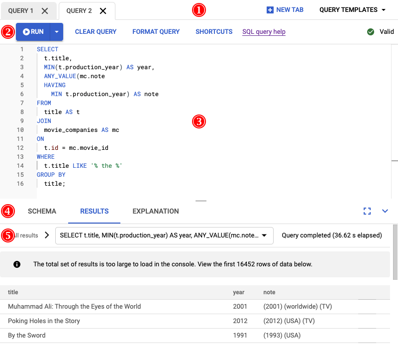
- The tab bar shows the query tabs you have open. To create a new
tab, click New tab.
The tab bar also provides a list of Query templates you can use to paste queries that provide insights about database queries, transactions, reads and more, as described in Overview of introspection tools.
- The editor commands bar provides these options:
- The Run command executes the statements entered in the
editing pane, producing query results in the Results tab and
query execution plans in the Explanation tab. Change the
default behavior using the drop down to produce Results only
or Explanation only.
Highlighting something in the editor changes the Run command to Run selected, allowing you to execute just what you have selected.
- The Clear query command deletes all text in the editor and clears the Results and Explanation subtabs.
- The Format query command formats statements in the editor so that they are easier to read.
- The Shortcuts command displays the set of keyboard shortcuts you can use in the editor.
- The SQL query help link opens a browser tab to documentation about SQL query syntax.
Queries are validated automatically any time they are updated in the editor. If the statements are valid, the editor commands bar displays a confirmation check mark and the message Valid. If there are any issues, it displays an error message with details.
- The Run command executes the statements entered in the
editing pane, producing query results in the Results tab and
query execution plans in the Explanation tab. Change the
default behavior using the drop down to produce Results only
or Explanation only.
- The editor is where you enter SQL query and DML statements.
They are color-coded and line numbers are automatically added for
multi-line statements.
If you enter more than one statement in the editor, you must use a terminating semicolon after each statement except the last one.
- The bottom pane of a query tab provides three subtabs:
- The Schema subtab shows the tables in the database and their schemas. Use it as a quick reference when composing statements in the editor.
- The Results subtab shows the results when you run the
statements in the editor. For queries it shows a results table, and
for DML statements like
INSERTand >UPDATEit shows a message about how many rows were affected. - The Explanation subtab shows visual graphs of the query plans created when you run the statements in the editor.
- The Results and Explanation subtabs both provide a statement selector you use to choose which statement's results or query plan you want to view.
View sampled query plans
- Go to the Spanner Instances page in Google Cloud console.
-
Click the name of the instance with the queries that you want to investigate.
Google Cloud console displays the instance's Overview page.
-
In the Navigation menu and under the Observability heading, click Query insights.
Google Cloud console displays the Instance's Query insights page.
-
In the Database drop-down menu, select the database with the queries you want to investigate.
Google Cloud console displays the query load information for the database. The TopN queries and tags table displays the list of top queries and request tags sorted by CPU utilization.
-
Find the query with high CPU utilization for which you want to view sampled query plans. Click the FPRINT value of that query.
The Query details page shows a Query plans samples graph for your query over time. You can zoom out to a maximum of seven days prior to the current time. Note: Query plans are not supported for queries with partitionTokens obtained from the PartitionQuery API and Partitioned DML queries.
-
Click one of the dots in the graph to see an older query plan and visualize the steps taken during the query execution. You can also click any operator to see expanded information about the operator.
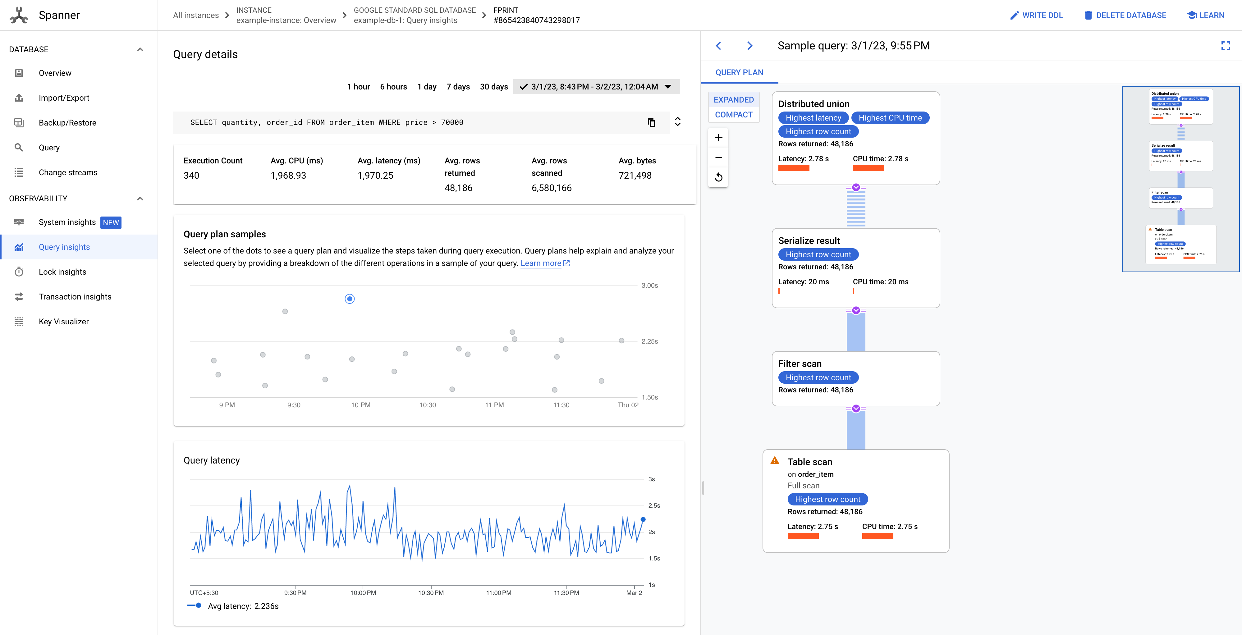
Figure 8. Query plan samples graph.
In some cases, you might want to view sampled query plans and compare the performance of a query over time. For queries that consume higher CPU, Spanner retains sampled query plans for 30 days on the Query insights page of the Google Cloud console. To view sampled query plans:
Take a tour of the query plan visualizer
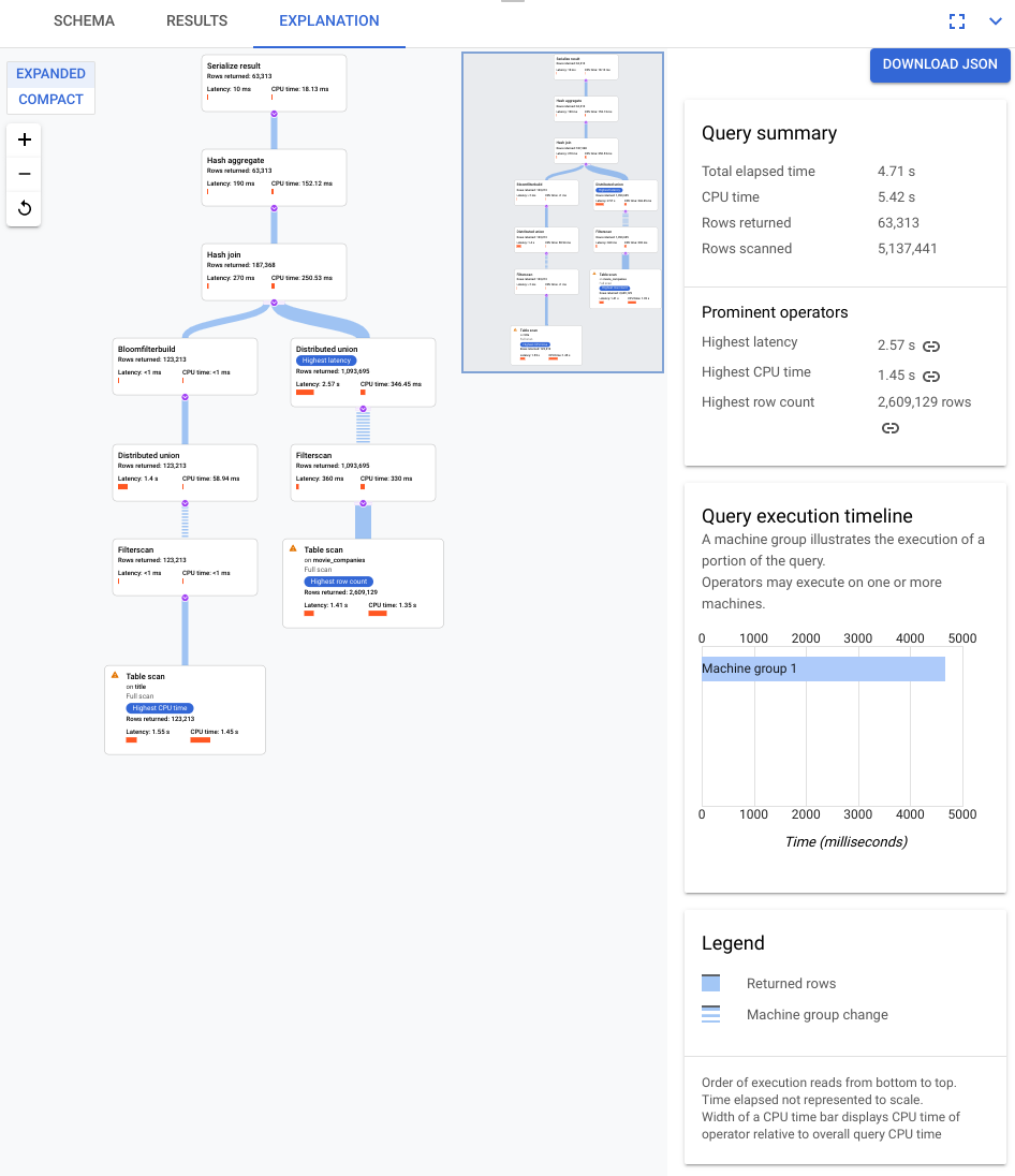
The key components of the visualizer are annotated in the following screenshot and described in more detail. After running a query in a query tab, select the EXPLANATION tab below the query editor to open the query execution plan visualizer.
The data flow in the following diagram is bottom-up, that is, all the tables and indexes are at the bottom of the diagram and the final output is at the top.
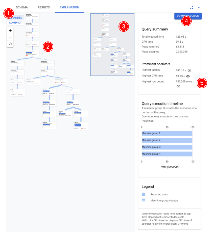
- The visualization of your plan can be large, depending on the query you executed. To hide and show details toggle the EXPANDED/COMPACT view selector. You can customize how much of the plan you see at any one time using the zoom control.
- The algebra that explains how Spanner runs the query
is drawn as an acyclic graph, where each node corresponds to an
iterator that consumes rows from its inputs and produces rows to its
parent. A sample plan is shown in Figure 9. Click the diagram
to see an expanded view of some of the details of the plan.
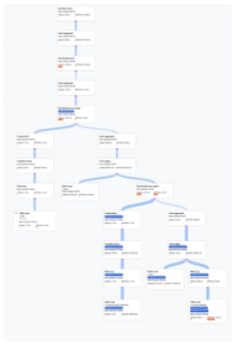
Figure 9. Sample visual plan (Click to zoom in). 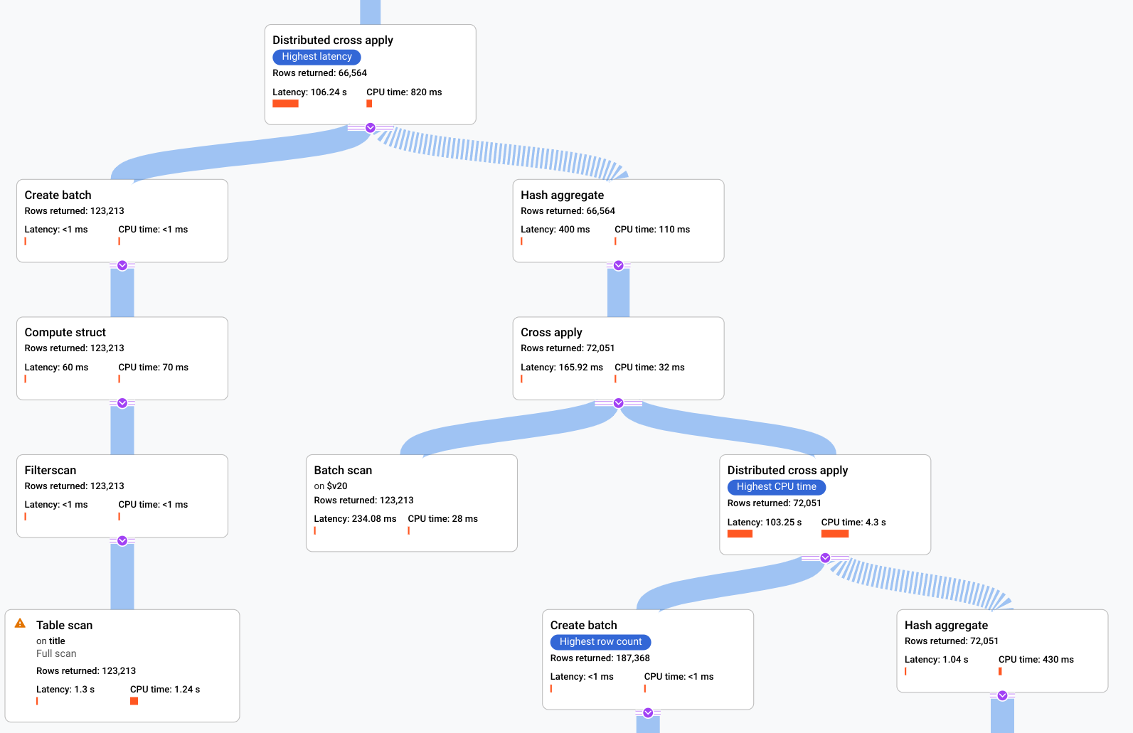
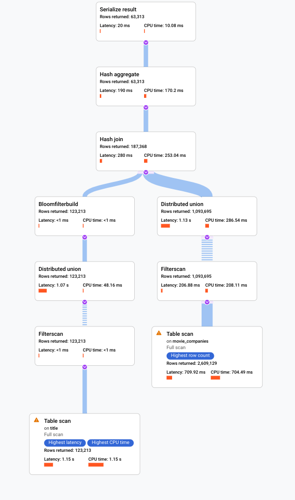
Each node, or card, on the graph represents an iterator and contains the following information:
- The iterator name. An iterator consumes rows from its input and produces rows.
- Runtime statistics telling you how many rows were returned, what the latency was, and how much CPU was consumed.
- We provide the following visual cues to help you identify potential issues within the query execution plan.
- Red bars in a node are visual indicators of the percentage of latency or CPU time for this iterator compared to the total for the query.
- The thickness of lines connecting each node represents the row count. The thicker the line, the larger the number of rows passed to the next node. The actual number of rows is displayed in each card and when you hold the pointer over a connector.
- A warning triangle is displayed on a node where a full table scan was performed. More details in the information panel include recommendations such as adding an index, or revising the query or schema in other ways if possible in order to avoid a full scan.
- Select a card in the plan to see details in the information panel on the right (5).
- The execution plan mini-map shows a zoomed-out view of the full plan and is useful for determining the overall shape of the execution plan and for navigating to different parts of the plan quickly. Drag directly on the mini-map or click where you'd like to focus, in order to go to another part of the visual plan.
Select DOWNLOAD JSON to download a JSON version of the execution plan, which is useful for troubleshooting. You can also share it when contacting the Spanner team for support. Saving the JSON doesn't save the result of the query.
To download and save a JSON version of the execution plan to visualize later:
- In Spanner Studio, run a query.
- Select the Explanation tab.
- Click DOWNLOAD JSON to download the JSON version of the execution plan.
- Save and copy the content of the JSON file.
- Open a new query editor tab.
- In the editor tab, enter:
  PROTO:
  CONTENT_OF_JSON
- Click Run.
- Select the Explanation tab below the query editor to view a visual representation of the downloaded execution plan.
- The information panel shows detailed contextual information about
the selected node in the query plan diagram. The information is
organized into the following categories.
- Iterator information provides details, as well as runtime statistics, for the iterator card you selected in the graph.
- Query summary provides details about the number of rows returned and the time it took to run the query. Prominent operators are those that exhibit significant latency, consume significant CPU relative to other operators, and return significant numbers of data rows.
- Query execution timeline is a time-based graph that shows how long each machine group was running its portion of the query. A machine group might not necessarily be running for the entire duration of the query's running time. It's also possible that a machine group ran multiple times during the course of running the query, but the timeline here only represents the start of the first time it ran and the end of the last time it ran.
Tune a query that exhibits poor performance
Imagine your company runs an online movie database that contains information about movies such as cast, production companies, movie details, and more. The service runs on Spanner, but has been experiencing some performance issues lately.
As lead developer for the service, you are asked to investigate these performance issues because they are causing poor ratings for the service. You open the Google Cloud console, go to your database instance and then open the query editor. You enter the following query into the editor and run it.
SELECT
  t.title,
  MIN(t.production_year) AS year,
  ANY_VALUE(mc.note HAVING MIN t.production_year) AS note
FROM
  title AS t
JOIN
  movie_companies AS mc
ON
  t.id = mc.movie_id
WHERE
  t.title LIKE '% the %'
GROUP BY
  title;
The result of running this query is shown in the following screenshot. We formatted the query in the editor by selecting FORMAT QUERY. There is also a note in the top right of the screen telling us that the query is valid.
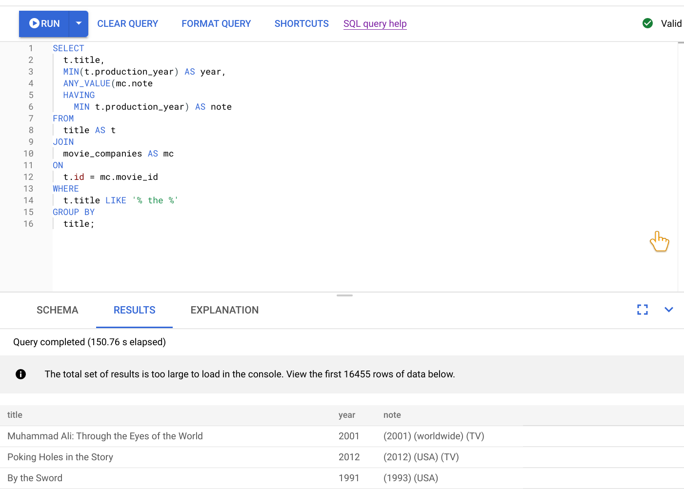
The RESULTS tab below the query editor shows that the query completed in just over two minutes. You decide to look closer at the query to see whether the query is efficient.
Analyze slow query with the query plan visualizer
At this point, we know that the query in the preceding step takes over two minutes, but we don't know whether the query is as efficient as possible and, therefore, whether this duration is expected.
You select the EXPLANATION tab just below the query editor to view a visual representation of the execution plan that Spanner created to run the query and return results.
The plan shown in the following screenshot is relatively large but, even at this zoom level, you can make the following observations.
Based on the Query summary in the information panel on the right, we learn that nearly 3 million rows were scanned and under 64K were ultimately returned.
We can also see from the Query execution timeline panel that 4 machine groups were involved in the query. A machine group is responsible for the execution of a portion of the query. Operators may execute on one or more machines. Selecting a machine group in the timeline highlights on the visual plan what part of the query was executed on that group.
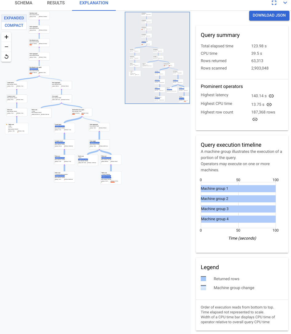
Because of these factors, you decide that an improvement in performance may be possible by changing the join from an apply join, which Spanner chose by default, to a hash join.
Improve the query
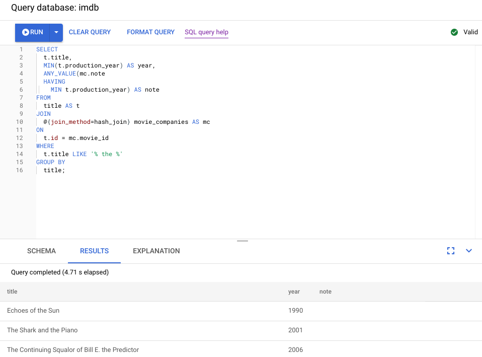
To improve the performance of the query, you use a join hint to change the join method to a hash join. This join implementation executes set-based processing.
Here's the updated query:
SELECT
  t.title,
  MIN(t.production_year) AS year,
  ANY_VALUE(mc.note HAVING MIN t.production_year) AS note
FROM
  title AS t
JOIN
  @{join_method=hash_join} movie_companies AS mc
ON
  t.id = mc.movie_id
WHERE
  t.title LIKE '% the %'
GROUP BY
  title;
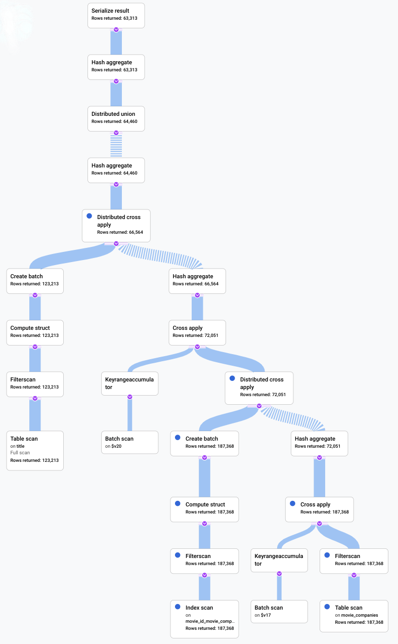
The following screenshot illustrates the updated query. As shown in the screenshot, the query completed in less than 5 seconds, a significant improvement over 120 seconds runtime before this change.
Examine the new visual plan, shown in the following diagram, to see what it tells us about this improvement.
Immediately, you notice some differences:
Only one machine group was involved in this query execution.
The number of aggregations has been reduced dramatically.
Conclusion
In this scenario, we ran a slow query and looked at its visual plan to look for inefficiencies. The following is a summary of the queries and plans before and after any changes were made. Each tab shows the query that was run and a compact view of the full query execution plan visualization.
Before
SELECT
  t.title,
  MIN(t.production_year) AS year,
  ANY_VALUE(mc.note
  HAVING
    MIN t.production_year) AS note
FROM
  title AS t
JOIN
  movie_companies AS mc
ON
  t.id = mc.movie_id
WHERE
  t.title LIKE '% the %'
GROUP BY
  title;
After
SELECT
  t.title,
  MIN(t.production_year) AS year,
  ANY_VALUE(mc.note
  HAVING
    MIN t.production_year) AS note
FROM
  title AS t
JOIN
  @{join_method=hash_join} movie_companies AS mc
ON
  t.id = mc.movie_id
WHERE
  t.title LIKE '% the %'
GROUP BY
  title;
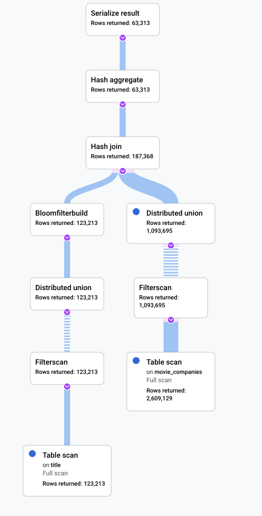
An indicator that something could be improved in this scenario was that a large
proportion of the rows from the table title qualified the filter LIKE
'% the %'. Seeking into another table with so many rows is likely to
be expensive. Changing our join implementation to a hash join improved
performance significantly.
What's next
For the complete query plan reference, refer to Query execution plans.
For the complete operator reference, refer to Query execution operators.