This page describes the techniques used to manipulate time-series data. This content builds on the concepts and discussion in Metrics, time series, and resources.
Raw time-series data must be manipulated before it can be analyzed, and analysis often involves filtering some data out and aggregating some together. This page describes two primary techniques for refining raw data:
- Filtering, which removes some of the data from consideration.
- Aggregation, which combines multiple pieces of data into a smaller set along dimensions you specify.
Filtering and aggregation are powerful tools to help identify interesting patterns and highlight trends or outliers in the data, among other things.
This page describes the concepts behind filtering and aggregation. It doesn't cover how to apply them directly. To apply filtering or aggregation to your time-series data, use the Cloud Monitoring API or the charting and alerting tools in the Google Cloud console. For examples, see API sample policies and Monitoring Query Language examples.Raw time-series data
The amount of raw metric data in a single time series can be enormous, and there are usually many time series associated with a metric type. To analyze the whole set of data for commonalities, trends, or outliers, you must do some processing on the time series in the set. Otherwise, there is too much data to consider.
To introduce filtering and aggregation the examples on this page use a small number of hypothetical time series. For example, the following illustration shows a few hours worth of raw data from three time series:
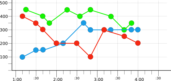
Each time series is colored, red, blue, or green, to reflect the value of a
hypothetical color label. There is one time series for each value of the
label. Notice that the values don't line up neatly, since they
were recorded at different times.
Filtering
One of the most powerful tools for analysis is filtering, which lets you hide data that isn't of immediate interest to you.
You can filter time-series data based on the following:
- Time.
- Value of one or more labels.
The following illustration shows the result of filtering to show only the red time series from the original set of raw time series (illustrated in Figure 1):

This time series, selected by filtering, is used in the next section, to demonstrate alignment.
Aggregation
Another way to reduce the amount of data you have is to summarize, or aggregate, it. There are two aspects to aggregation:
- Alignment, or regularizing data within a single time series.
- Reduction, or combining multiple time series.
You must align time series before you can reduce them. The next few
sections describe alignment and reduction by using time series that store
integer values. These general concepts also apply when a time series has a
Distribution value type; however, there are some
additional constraints in this case. For more information, see
About distribution-valued metrics.
Alignment: within-series regularization
The first step in aggregating time-series data is alignment. Alignment creates a new time series in which the raw data has been regularized in time so it can be combined with other aligned time series. Alignment produces time series with regularly spaced data.
Alignment involves two steps:
Dividing the time series into regular time intervals, also called bucketing the data. The interval is called the period, alignment period, or alignment window.
Computing a single value for the points in the alignment period. You choose how that single point is computed; you might sum all the values, or compute their average, or use the maximum.
Because the new time series created by alignment represents all the values from the raw time series that are within the alignment period with a single value, it is also called within-series reduction or within-series aggregation.
Regularizing time intervals
Analyzing time-series data requires that the data points be available on evenly spaced time boundaries. Alignment is the process for making this happen.
Alignment creates a new time series with a constant interval, the alignment period, between data points. Alignment is typically applied to multiple time series in preparation for further manipulation.
This section illustrates the alignment steps by applying them to a single time series. In this example, a one-hour alignment period is applied to the example time series illustrated in Figure 2. The time series shows data captured over three hours. Breaking the data points into one-hour periods results in the following points in each period:
| Period | Values |
|---|---|
| 1:01–2:00 | 400, 350, 300, 200 |
| 2:01–3:00 | 200, 100 |
| 3:01–4:00 | 300, 250, 200 |
Choosing alignment periods
The duration of the alignment period depends on two factors:
- The granularity of what you are trying to find in the data.
- The sampling period of the data; that is, how often it is reported.
The following sections discuss these factors in more detail.
Also, Cloud Monitoring keeps metric data for a finite period of time. The period varies with the metric type; see Data retention for details. The retention period is the longest meaningful alignment period.
Granularity
If you know that something happened within a span of a couple of hours, and you want to dig deeper, you probably want to use a period of an hour or some number of minutes for alignment.
If you are interested in exploring trends over longer periods of time, a larger alignment period may be more appropriate. Large alignment periods are typically not useful for looking at short-term anomalous conditions. If you use, for example, a multi-week alignment period, the existence of an anomaly in that period may still be detectable, but the aligned data might be too coarse-grained to be much help.
Sampling rate
The frequency with which the data is written, the sampling rate, can also affect the choice of alignment period. See Metrics list for the sampling rates of built-in metrics. Consider the following figure, which illustrates a time series with a sampling rate of one point per minute:
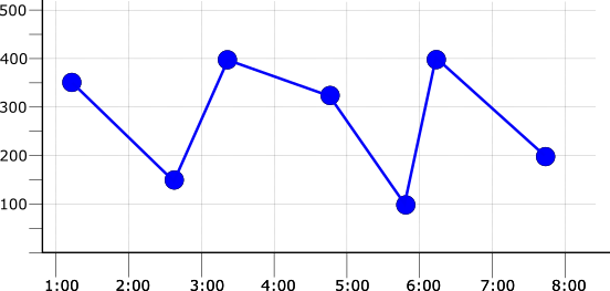
If the alignment period is the same as the sampling period, then
there is one data point in each alignment period. This means that, for
example, applying any of the max, mean, or min aligners
results in the same aligned time series. The following illustration shows
this result, along with the original time series as a faded line:

For more information about how aligner functions work, see Aligners.
If the alignment period is set to two minutes, or double the sampling
period, then there are two data points in each period. If the max, mean,
or min aligners are applied to the points within the two-minute alignment
period, the resulting time series differ. The following illustration shows
these results, along with the original time series as a faded line:

When choosing an alignment period, make it longer than the sampling period, but short enough to show relevant trends. You might have to experiment to determine a useful alignment period. For example, if data is collected at the rate of one point per day, an alignment period of an hour is too short to be useful: for most hours, there will be no data.
Aligners
After the data is broken into alignment periods, you select a function, the aligner, to be applied to the data points in that period. The aligner produces a single value placed at the end of each alignment period.
Alignment options include summing the values, or finding the max, min, or
mean of the values, finding a chosen percentile value, counting the values, and
others. The Cloud Monitoring API supports a large set of alignment functions,
many more than the set illustrated here; see Aligner
for the full list. For a description of rate and delta aligners,
which transform time series data, see
Kinds, types, and conversions.
For example, taking the bucketed data from the raw time series (illustrated in Figure 1), choose an aligner and apply it to the data in each bucket. The following table shows the raw values and the results of three different aligners, max, mean, and min:
| Period | Values | Aligner: max | Aligner: mean | Aligner: min |
|---|---|---|---|---|
| 1:01–2:00 | 400, 350, 300, 200 | 400 | 312.5 | 200 |
| 2:01–3:00 | 200, 100 | 200 | 150 | 100 |
| 3:01–4:00 | 300, 250, 200 | 300 | 250 | 200 |
The following illustration shows the results of applying the max, mean, or min aligners using a 1-hour alignment period to the original red time series (represented by the faded line in the illustration):

Some other aligners
The following table shows the same raw values and the results of three other aligners:
- Count counts the number of values in the alignment period.
- Sum adds up all the values in the alignment period.
- Next older uses the most recent value in the period as the alignment value.
| Period | Values | Aligner: count | Aligner: sum | Aligner: next older |
|---|---|---|---|---|
| 1:01–2:00 | 400, 350, 300, 200 | 4 | 1250 | 200 |
| 2:01–3:00 | 200, 100 | 2 | 300 | 100 |
| 3:01–4:00 | 300, 250, 200 | 3 | 750 | 200 |
These results are not shown on a chart.
Reduction: combining time series
The next step in the process, reduction, is the process of combining multiple aligned time series into a new time series. This step replaces all the values on the alignment-period boundary with a single value. Because it works across separate time series, reduction is also called cross-series aggregation.
Reducers
A reducer is a function that is applied to the values across a set of time series to produce a single value.
Reducer options include summing the aligned values, or finding the max, min,
or mean of the values. The Cloud Monitoring API supports a large set of
reduction functions; see Reducer for the full list.
The list of reducers parallels the list of aligners.
Time series must be aligned before they can be reduced. The following illustration shows the results aligning all three of the raw time series (from Figure 1) into 1-hour periods with the mean aligner:
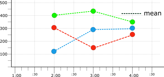
The values from the three mean-aligned time series (illustrated in Figure 4) are shown in the following table:
| Alignment boundary | Red | Blue | Green |
|---|---|---|---|
| 2:00 | 312.5 | 133.3 | 400 |
| 3:00 | 150 | 283.3 | 433.3 |
| 4:00 | 250 | 300 | 350 |
Using the aligned data in the preceding table, choose a reducer and apply it to the values. The following table shows the results of applying different reducers to the mean-aligned data:
| Alignment boundary | Reducer: max | Reducer: mean | Reducer: min | Reducer: sum |
|---|---|---|---|---|
| 2:00 | 400 | 281.9 | 133.3 | 845.8 |
| 3:00 | 433.3 | 288.9 | 150 | 866.7 |
| 4:00 | 350 | 300 | 250 | 900 |
By default, reduction applies across all your time series, resulting in a single time series. The following illustration shows the result of aggregating the three mean-aligned time series with the max reducer, which yields the highest mean values across the time series:
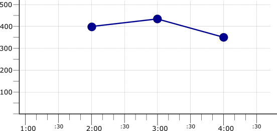
Reduction can also be combined with grouping, in which time series are organized into categories, and the reducer is applied across the time series in each group.
Grouping
Grouping lets you apply a reducer across subsets of your time series rather than across the entire set of time series. To group time series, you select one or more labels. The time series are then grouped on the basis of their values for the selected labels. Grouping results in one time series for each group.
If a metric type records values for zone and color labels,
you can group time series by either or both labels. When you apply the
reducer, each group is reduced to a single time series. If you group
by color, you get one time series for each color represented in the data.
If you group by zone, you get a time series for each zone that appears
in the data. If you group by both, you get a time series for each combination
of colors and zones.
For example, suppose you have captured many time series with “red,”
“blue,” and “green” values for the color label. After
aligning all the time series, they can be grouped by color value and then
reduced by group. This results in three color-specific time series:
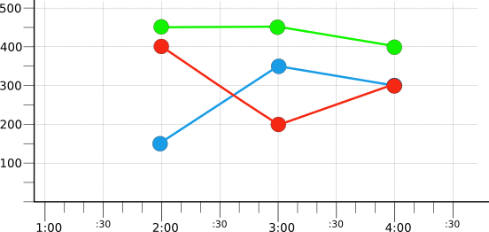
The example does not specify the aligner or reducer used; the point here is
that grouping lets you reduce a large set of time series into a smaller set,
where each time series represents a group sharing a common attribute: in this
example, the value of the color label.
Secondary aggregation
Cloud Monitoring performs two aggregation steps.
Primary aggregation regularizes the measured data and then combines the regularized time series by using a reducer. When you use grouping, more than one time series might result from the reduction performed as part of the this step.
Secondary aggregation, which applies to the results of the primary aggregation step, lets you combine the grouped time series into one result by using a second reducer.
The following table shows the values of the grouped time series (illustrated in Figure 6):
| Alignment boundary | Red group | Blue group | Green group |
|---|---|---|---|
| 2:00 | 400 | 150 | 450 |
| 3:00 | 200 | 350 | 450 |
| 4:00 | 300 | 300 | 400 |
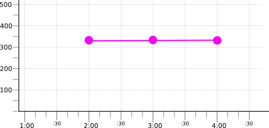
These three already-reduced time series can then be further reduced by applying secondary aggregation. The following table shows the results of applying selected reducers:
| Alignment boundary | Reducer: max | Reducer: mean | Reducer: min | Reducer: sum |
|---|---|---|---|---|
| 2:00 | 450 | 333.3 | 150 | 1000 |
| 3:00 | 450 | 333.3 | 200 | 1000 |
| 4:00 | 400 | 333.3 | 300 | 1000 |
The following illustration shows the result of aggregating the three grouped series with the mean reducer:
Kinds, types, and conversions
Recall that the data points in a time series are characterized by a metric kind and a value type; see Value types and metric kinds for a review. The appropriate aligners and reducers for one set of data might not be appropriate for another. For example, an aligner or reducer that counts the number of false values is appropriate for boolean data but not for numeric data. Likewise, an aligner or reducer that computes a mean is applicable to numeric data but not to boolean data.
Some aligners and reducers can also be used to explicitly change either the
metric kind or the value type of data in a time series. Some, such as
ALIGN_COUNT, do so as a side effect.
Metric kind: A cumulative metric is one in which each value represents the total since collection of values began. You can't use cumulative metrics directly in charts, but you can use delta metrics, in which each value represents the change since the previous measurement.
You can also convert both cumulative and delta metrics to gauge metrics. For example, consider a delta metric whose time series is as follows:
(start time, end time] (minutes) value (MiB) (0, 2] 8 (2, 5] 6 (6, 9] 9 Assume that you selected an aligner of
ALIGN_DELTAand an alignment period of three minutes. Because the alignment period doesn't match the (start time, end time] for each sample, a time series is created with interpolated values. For this example, the interpolated time series is:(start time, end time] (minutes) interpolated value (MiB) (0, 1] 4 (1, 2] 4 (2, 3] 2 (3, 4] 2 (4, 5] 2 (5, 6] 0 (6, 7] 3 (7, 8] 3 (8, 9] 3 Next, all of the points within the three-minute alignment period are summed to generate the aligned values:
(start time, end time] (minutes) aligned value (MiB) (0, 3] 10 (3, 6] 4 (6, 9] 9 If
ALIGN_RATEis selected, the process is the same except that the aligned values are divided by the alignment period. For this example, the alignment period is three minutes so the aligned time series has the following values:(start time, end time] (minutes) aligned value (MiB / second) (0, 3] 0.056 (3, 6] 0.022 (6, 9] 0.050 To chart a cumulative metric, it must be converted to a delta metric or a rate metric. The process for cumulative metrics is similar to the previous discussion. You can compute a delta time series from a cumulative time series by computing the difference of adjacent terms.
Value type: Some aligners and reducers leave the value type of the input data unchanged; for example, integer data is still integer data after alignment. Other aligners and reducers convert data from one type to another, which means the information can be analyzed in ways not appropriate to the original value type.
For example, the
REDUCE_COUNTreducer can be applied to numeric, boolean, string, and distribution data, but the result it produces is a 64-bit integer counting the number of values in the period.REDUCE_COUNTcan be applied only to gauge and delta metrics, and it leaves the metric kind unchanged.
The reference tables for Aligner and
Reducer
indicate what kind of data each is appropriate for and any conversion that
results. For example, the following shows the entry for ALIGN_DELTA:

