Improve query performance by using Query Insights

Preview

This product is covered by the Pre-GA Offerings Terms of the Google Cloud Terms of Service. Pre-GA products might have limited support, and changes to pre-GA products might not be compatible with other pre-GA versions. For more information, see the launch stage descriptions.

This page describes how to use the Query Insights dashboard to detect and analyze performance problems. For an overview of this feature, see Query Insights overview.

Before you begin

If you or other users need to view the query plan or perform end-to-end tracing, you need specific IAM permissions to do so. You can create a custom role and add the necessary IAM permissions to it. Then, you can add this role to each user account that will use Query Insights to troubleshoot an issue. See Create a custom role.

The custom role needs to have the following IAM permission: cloudtrace.traces.get.

Open the Query Insights dashboard

Preview — Gemini in Databases

This feature is subject to the "Pre-GA Offerings Terms" in the General Service Terms section of the Service Specific Terms. You can process personal data for this feature as outlined in the Cloud Data Processing Addendum, subject to the obligations and restrictions described in the agreement under which you access Google Cloud. Pre-GA features are available "as is" and might have limited support. For more information, see the launch stage descriptions.

To open the Query Insights dashboard, do the following steps:

1. From the list of clusters and instances, click an instance.
2. Either click Go to Query Insights for more in-depth info on queries and performance below the metrics graph on the cluster Overview page or select the Query Insights tab in the left navigation panel.

On the subsequent page, you can use the following options to filter the results:

1. Instance selector. Lets you select either the primary instance or read pool instances in the cluster. By default, the primary instance is selected. The details shown are aggregated for all connected read pool instances and their nodes.
2. Database. Filters query load on a specific database or all databases.
3. User. Filters query load from specific user accounts.
4. Client address. Filters query load from a specific IP address.
5. Time range. Filters query load by time ranges, such as hour, day, week, or a custom range.

Note: If you enable Gemini in Databases, the data retention policy for query metrics is 30 days.

Edit the Query Insights configuration

Query Insights is enabled by default on AlloyDB instances. You can edit the default Query Insights configuration.

To edit the Query Insights configuration for an AlloyDB instance, follow these steps:

Console

1. In the Google Cloud console, go to the Clusters page.

   Go to Clusters

2. Click a cluster in the Resource Name column.

3. Click Query Insights in the left navigation panel.

4. Select Primary or Read pool from the Query Insights list, and then click Edit.

5. Edit the Query Insights fields:

   1. To change the default limit of 1024 bytes on query lengths for AlloyDB to analyze, in the Customize query lengths field, enter a number from 256 to 4500.

      The instance restarts after you edit this field.

      Note: Higher query-length limits require more memory.

   2. To customize your Query Insights feature sets, adjust the following options:

      • Enable query plans. Set this checkbox to know the operations used to execute a sample of a query.
        In the Maximum sampling rate field, enter a number from 1 to 20. By default, the sampling rate is set to 5. To disable sampling, clear the Enable query plans checkbox.
        The sampling rate determines the maximum number of queries that AlloyDB can sample per minute for the instance per node.
      • Store client IP addresses. Set this checkbox to know from where your queries are originating, and to group that information to run metrics.
      • Store application tags. Set this checkbox to know which tagged applications are making requests, and to group that information to run metrics. For more information about application tags, see the specification .

6. Click Update instance.

gcloud

gcloud alloydb instances update INSTANCE \
--cluster=CLUSTER \
--project=PROJECT \
--region=REGION \
--insights-config-query-string-length=QUERY_LENGTH \
--insights-config-query-plans-per-minute=QUERY_PLANS} \
--insights-config-record-application-tags \
--insights-config-record-client-address

Replace the following:

• CLUSTER: the ID of the instance to update
• CLUSTER: the ID of the instance's cluster
• PROJECT: the ID of the cluster's project
• REGION: the cluster's region—for example, us-central1
• QUERY_LENGTH: the length of the query that ranges from 256 to 4500
• QUERY_PLANS: the number of query plans to configure per minute

Also, use one or more of the following optional flags:

• --insights-config-query-string-length: Sets the default query length limit to a specified value from 256 to 4500 bytes. The default query length is 1024 bytes. Higher query lengths are more useful for analytical queries, but they also require more memory. Changing the query length requires you to restart the instance. You can still add tags to queries that exceed the length limit.
• --insights-config-query-plans-per-minute: By default, a maximum of five executed query plan samples are captured per minute across all databases on the instance. Change this value to a number from 1 to 20. To disable sampling, enter 0. Increasing the sampling rate is likely to give you more data points but might add a performance overhead.
• --insights-config-record-client-address: Stores the client IP addresses where queries are coming from and helps you group that data to run metrics against it. Queries come from more than one host. Reviewing graphs for queries from client IP addresses can help identify the source of a problem. If you do not wish to store client IP addresses, use --no-insights-config-record-client-address.
• --insights-config-record-application-tags: Stores application tags that help you determine the APIs and model-view-controller (MVC) routes that are making requests and group the data to run metrics against it. This option requires you to comment queries with a specific set of tags. If you do not wish to store application tags, use --no-insights-config-record-application-tags.

Steps to improve query performance

Query Insights troubleshoots AlloyDB queries to look for performance issues. The Query Insights dashboard shows the query load based on factors that you select. Query load is a measurement of the total work for all the queries in the instance in the selected time range.

Query Insights helps you detect and analyze query performance problems. You use Query Insights to troubleshoot queries in four steps:

1. View the database load for all queries.
2. Identify a potentially problematic query or tag.
3. Examine the query or tag to identify issues.
4. Trace the source of the problem.

View the database load for all queries

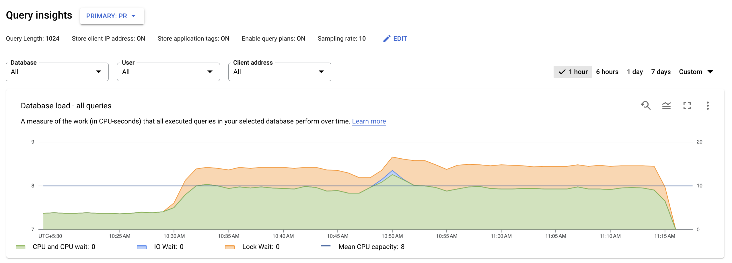
The top-level Query Insights dashboard shows the Database load — all top queries graph using filtered data. Database query load is a measure of the work (in CPU seconds) that the executed queries in your selected database perform over time. Each running query is either using or waiting for CPU resources, IO resources, or lock resources. Database query load is the ratio of the amount of time taken by all the queries that are completed in a given time window to the wall clock time.

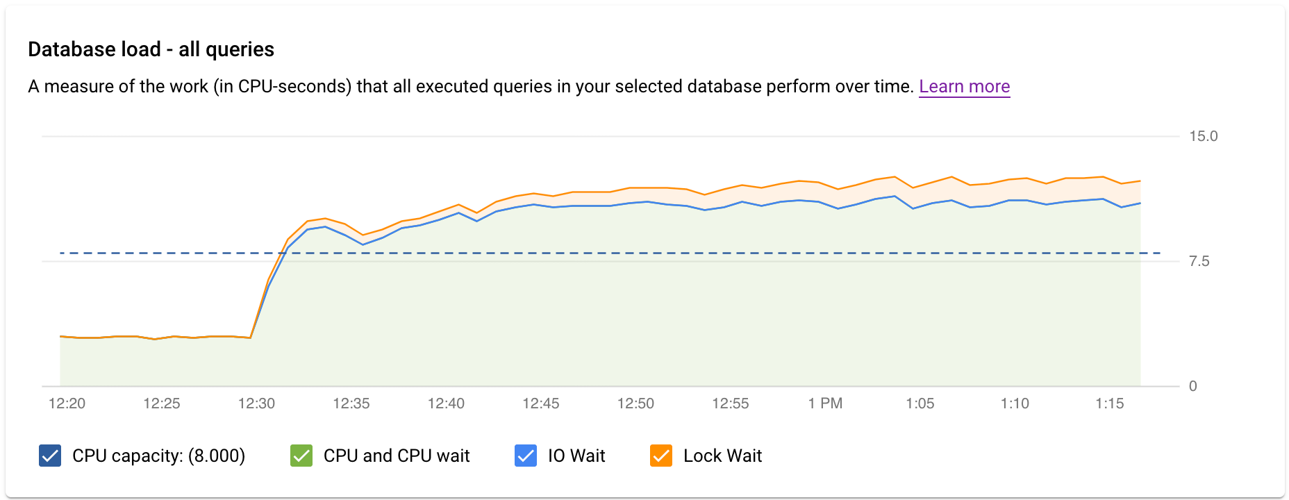
Colored lines in the graph show the query load, split into four categories:

• CPU capacity: The number of CPUs available on the instance.

• CPU and CPU Wait: The ratio of the time taken by queries in an active state to wall clock time. IO and Lock waits do not block queries that are in an active state. This metric might mean that the query is either using the CPU or waiting for the Linux scheduler to schedule the server process running the query while other processes are using the CPU.

  Note: CPU load accounts for both the runtime and the time waiting for the Linux scheduler to schedule the server process that is running. As a result, the CPU load can go beyond the maximum core line.

• IO Wait: The ratio of time taken by queries that are waiting for IO to wall clock time. IO wait includes Read IO Wait and Write IO Wait. See the PostgreSQL event table. If you want a breakdown of information for IO waits, you can see it in Cloud Monitoring. For more information, see metrics charts.

• Lock Wait: The ratio of time taken by queries that are waiting for Locks to wall clock time. It includes Lock Waits, LwLock Waits, and Buffer pin Lock waits. If you want a breakdown of information for lock waits, you can see it in Cloud Monitoring. For more information, see metrics charts.

Next, review the graph and use the filtering options to answer these questions:

1. Is the query load high? Is the graph spiking or elevated over time? If you don't see a high load, then the problem isn't with your queries.
2. How long has the load been high? Is it only high now? Or has it been high for a long time? Use the range selection to select various time periods to find out how long the problem has occurred. Or you can zoom in to view a time window where query load spikes are observed. You can zoom out to view up to one week of the timeline.
3. What is causing the high load? You can select options to look at the CPU capacity, CPU and CPU wait, lock wait, or IO wait. The graph for each of these options is a different color so that you can see which one has the highest load. The dark blue line on the graph shows the max CPU capacity of the system. It lets you compare the query load with the max CPU system capacity. This comparison helps you know whether an instance is running out of CPU resources.
4. Which database is experiencing the load? Select different databases from the Databases drop-down menu to find the databases with the highest loads.
5. Are specific users or IP addresses causing higher loads? Select different users and addresses from the drop-down menus to compare which ones are causing higher loads.

Filter the database load

The Queries and tags sections lets you filter or sort the query load for either a selected query or a SQL query tag.

Filter by queries

The QUERIES table provides an overview of the queries that cause the most query load. The table shows all the normalized queries for the time window and options selected on the Query Insights dashboard.

By default, the table sorts queries by the total execution time within the time window you selected.

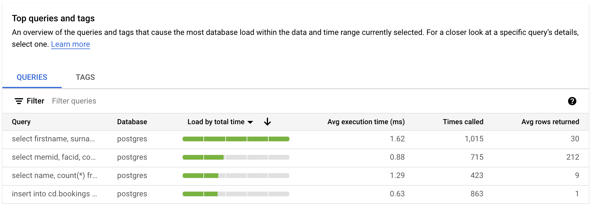
To filter the table, select a property from Filter queries. To sort the table, select a column heading. The table shows the following properties:

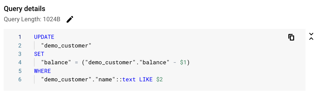
• Query string. The normalized query string. Query Insights only shows 1024 characters in the query string by default.

  Queries labeled UTILITY COMMAND usually include BEGIN, COMMIT, and EXPLAIN commands or wrapper commands.

• Database. The database that the query was run against.

• Load by total time/Load by CPU/Load by IO wait/Load by lock wait. These options let you filter specific queries to find the largest load for each option.

• Avg execution time (ms). The total time that all sub-tasks take across all parallel workers to complete the query. For more information, see Average execution time and duration.

• Times called. The number of times the query was called by the application.

• Avg rows fetched. The average number of rows fetched for the query.

Query Insights displays normalized queries, that is, $1, $2, and so on replace the literal constant values. For example:

UPDATE
  "demo_customer"
SET
  "customer_id" = $1::uuid,
  "name" = $2,
  "address" = $3,
  "rating" = $4,
  "balance" = $5,
  "current_city" = $6,
  "current_location" = $7
WHERE
  "demo_customer"."id" = $8

The constant's value is ignored so that Query Insights can aggregate similar queries and remove any PII information that the constant might show.

Filter by query tags

To troubleshoot an application, you must first add tags to your SQL queries.

Query Insights provides application-centric monitoring to diagnose performance problems for applications built using ORMs.

If you're responsible for the entire application stack, Query Insights provides query monitoring from an application view. Query tagging helps you find issues at higher-level constructs, such as using the business logic, a microservice, or some other construct. You might tag queries by the business logic, for example, using the payment, inventory, business analytics, or shipping tags. You can then find the query load that the various business logics create. For example, you might find unexpected events, such as spikes for a business analytics tag at 1 PM. Or you might see abnormal growth for a payment service trending over the previous week.

Query load tags provide a breakdown of the query load of the selected tag over time.

To calculate the Database Load for Tag, Query Insights uses the amount of time taken by every query that uses the tag you select. Query Insights calculates the completion time at the minute boundary using wall clock time.

On the Query Insights dashboard, select TAGS to view the tags table. The TAGS table sorts tags by their total load by total time.

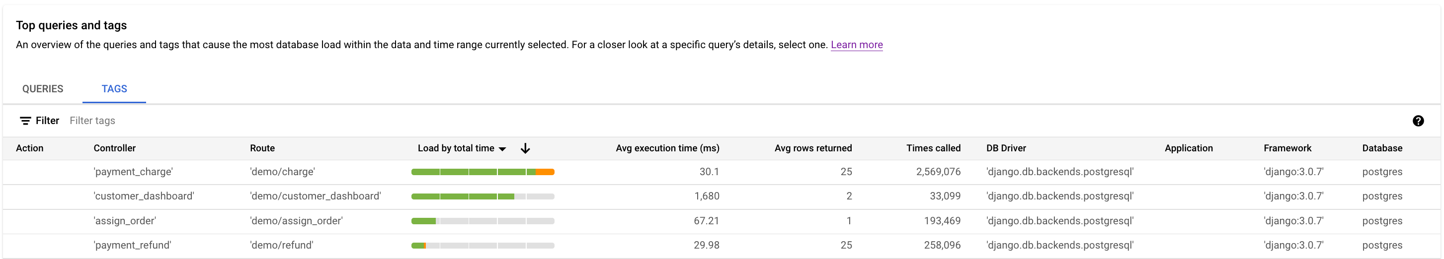
You can sort the table by selecting a property from Filter queries, or by clicking a column heading. The table shows the following properties:

• Action, Controller, Framework, Route, Application, DB Driver. Each property that you added to your queries is shown as a column. At least one of these properties must be added if you want to filter by tags.
• Load by total time/Load by CPU/Load by IO wait/Load by lock wait. These options let you filter specific queries to find the largest load for each option.
• Avg execution time (ms). The total time that all sub-tasks take across all parallel workers to complete the query. For more information, see Average execution time and duration.
• Times called. The number of times the query was called by the application.
• Avg rows fetched. The average number of rows fetched for the query.
• Database. The database that the query was run against.

Examine a specific query or tag

To determine if a query or a tag is the root cause of the problem, do the following from the Queries tab or Tags tab, respectively:

1. Click the Load by total time header to sort the list in descending order.
2. Click the query or tag that looks like it has the highest load and is taking a longer time than the others.

A dashboard opens showing the details of the selected query or tag.

If you selected a query, an overview of the selected query is shown:

If you selected a tag, an overview of the selected tag is shown.

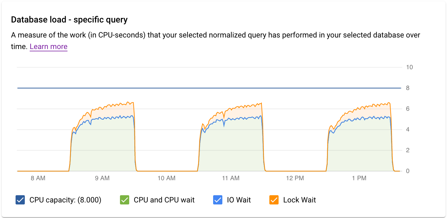
Examine the load for a specific query or tag

The Database load — specific query graph shows a measure of the work (in CPU seconds) that your selected normalized query has performed in your selected query over time. To calculate load, it uses the amount of time taken by the normalized queries that are completed at the minute boundary to the wall clock time. At the top of the table, the first 1024 characters of the normalized query (where literals are removed for aggregation and PII reasons) are displayed. As with the total queries graph, you can filter the load for a specific query by Database, User, and Client Address. Query load is split into CPU capacity, CPU and CPU Wait, IO Wait, and Lock Wait.

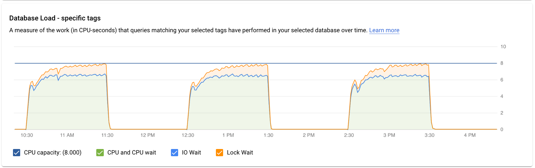
The Database load — specific tags graph shows a measure of the work (in CPU seconds) that queries matching your selected tags have performed in your selected database over time. As with the total queries graph, you can filter the load for a specific tag by Database, User, and Client Address.

Examine the latency

You use the Latency graph to examine latency on the query or tag. Latency is the time taken for the normalized query to complete, in wall clock time. The latency dashboard shows 50th, 95th, and 99th percentile latency to find outlier behaviors.

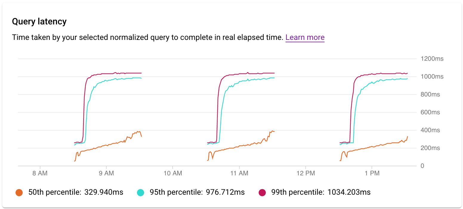
The latency of Parallel Queries is measured in wall clock time even though query load can be higher for the query due to multiple cores being used to run part of the query.

Try to narrow down the problem by looking at the following:

1. What is causing the high load? Select options to look at the CPU capacity, CPU and CPU wait, lock wait, or IO wait.
2. How long has the load been high? Is it only high now? Or has it been high for a long time? Change the time ranges to find the date and time that the load started performing poorly.
3. Were there spikes in latency? You can change the time window to study the historical latency for the normalized query.

When you find the areas and times for the highest load, you can drill down further.

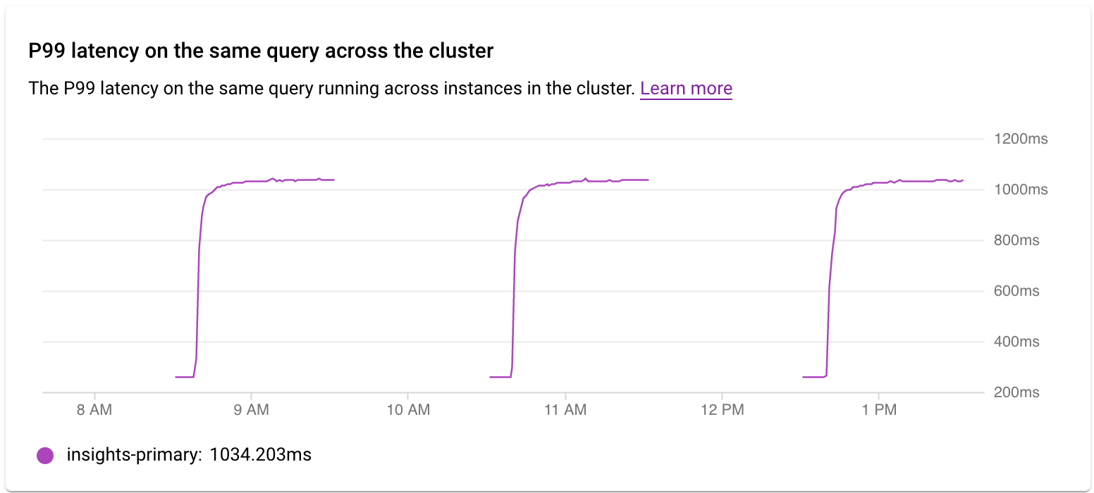
Examine the latency across a cluster

You use the P99 latency on the same query across the cluster graph to examine P99 latency on the query or tag across instances in the cluster.

Examine operations in a sampled query plan

A query plan takes a sample of your query and breaks it down into individual operations. It explains and analyzes each operation in the query. The Query plan samples graph shows all the query plans running at particular times and the amount of time each plan took to run.

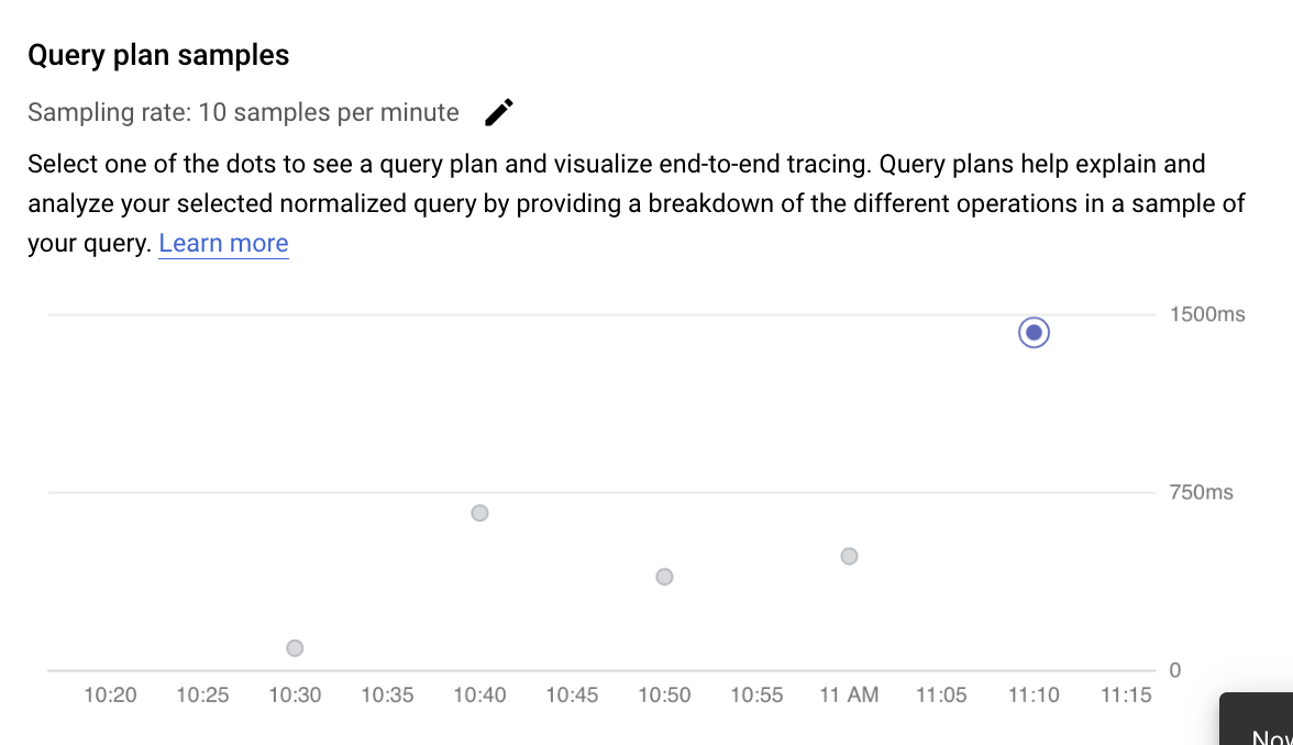
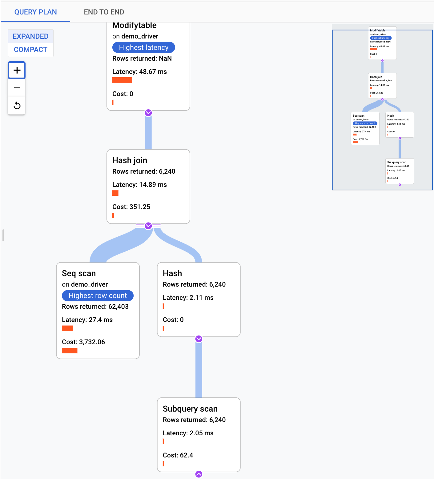
To see details for the sample query plan, click the dots on the Sample query plans graph. There is a view of executed sample query plans for most, but not all, queries. Expanded details show a model of all the operations in the query plan. Each operation shows the latency, rows returned, and the cost for that operation. When you select an operation, you can see more details, such as shared hit blocks, the type of schema, the actual loops, plan rows, and more.

Try to narrow down the problem by looking at the following questions:

1. What is the resource consumption?
2. How does it relate to other queries?
3. Does consumption change over time?

Trace the source of the problem

To help you identify the specific source of the problem, such as a specific model, view, controller, route, host, or user, Query Insights provides an in-context end-to-end application trace view to understand what's going on at the database layer for a specific request and to find the source of a problematic query by model, view, controllers, and route. If you enable OpenCensus or OpenTelemetry, opencensus span information is sent to the database along with the tag information inside SQL comments. Any traces from the application to Cloud Logging are linked with database query plan traces to identify the source of the problem. You can click the END to END tab in the Sample Query screen to look at the in-context trace.

To determine the client and user causing the problem, use the Top Client addresses and Top Users tables to find the highest loads. You can add a user or IP address to the filter to further analyze a specific user or client address.

For queries, you can use Cloud Trace to see end-to-end tracing for each step in the query plan. On the Query Insights dashboard, click the View in trace link to open the Cloud Trace tool.

For details about how to use tools in Cloud Trace, see Finding and viewing traces.

Add tags to SQL queries

Tagging SQL queries simplifies application troubleshooting. You can use sqlcommenter to add tags to your SQL queries either automatically by using Object-relational mapping (ORM) or manually.

Use sqlcommenter with ORM

When ORM is used instead of directly writing SQL queries, you might not find application code that is causing performance challenges. You might also have trouble analyzing how your application code impacts query performance. To tackle that pain point, Query Insights provides an open source library called sqlcommenter, an ORM instrumentation library. This library is useful for developers using ORMs and administrators to detect which application code is causing performance problems.

If you're using ORM and sqlcommenter together, the tags are auto created without requiring you to change or add custom code to your application.

You can install sqlcommenter on the application server. The instrumentation library allows application information related to your MVC framework to be propagated to the database along with the queries as a SQL comment. The database picks up these tags and starts recording and aggregating statistics by tags, which are orthogonal with statistics aggregated by normalized queries. Query Insights shows the tags so that you know which application is causing the query load. This information helps you find which application code is causing performance problems.

When you examine results in SQL database logs, they appear as follows:

SELECT * from USERS /*action='run+this',
controller='foo%3',
traceparent='00-01',
tracestate='rojo%2'*/

Supported tags include the controller name, route, framework, and action.

The set of ORMs in sqlcommenter is supported for various programming languages:

Python	Django psycopg2 Sqlalchemy Flask
Java	Hibernate Spring
Ruby	Rails
Node.js	Knex.js Sequelize.js Express.js

For more information about sqlcommenter and how to use it sqlcommenter in your ORM framework, see the sqlcommenter documentation in GitHub.

Use sqlcommenter to add tags manually

If you're not using ORM, you must manually add sqlcommenter tags to your SQL queries. In your query, you must augment each SQL statement with a comment containing a serialized key-value pair. Use at least one of the following keys:

• action=''
• controller=''
• framework=''
• route=''
• application=''
• db driver=''

Query Insights drops all other keys. See the sqlcommenter documentation for the correct SQL comment format.

Execution time and duration

Query Insights provides an Avg execution time (ms) metric, which reports the total time that all sub-tasks take across all parallel workers to complete the query. This metric can help you optimize the aggregate resource utilization of databases by finding and optimizing queries that create the highest CPU overhead.

To view the elapsed time, you can measure the duration of a query by running the \timing command on the psql client. It measures the time that elapses between receiving the query and the PostgreSQL server sending a response. This metric can help you analyze why a given query is taking too long, and decide whether to optimize it to run faster.

If a query is completed single-threaded by a single task, the duration and average execution time remain the same.

What's Next

• Query Insights overview
• AlloyDB metrics
• SQL Commenter blog: Introducing Sqlcommenter: An open source ORM auto-instrumentation library
• How-to blog: Enable query tagging with Sqlcommenter