Use Apache Beam notebook advanced features

Using the Apache Beam interactive runner with JupyterLab notebooks lets you iteratively develop pipelines, inspect your pipeline graph, and parse individual PCollections in a read-eval-print-loop (REPL) workflow. For a tutorial that demonstrates how to use the Apache Beam interactive runner with JupyterLab notebooks, see Develop with Apache Beam notebooks.

This page provides details about advanced features that you can use with your Apache Beam notebook.

Interactive FlinkRunner on notebook-managed clusters

To work with production-sized data interactively from the notebook, you can use the FlinkRunner with some generic pipeline options to tell the notebook session to manage a long-lasting Dataproc cluster and to run your Apache Beam pipelines distributedly.

Prerequisites

To use this feature:

• Enable the Dataproc API.
• Grant an admin or editor role to the service account that runs the notebook instance for Dataproc.
• Use a notebook kernel with the Apache Beam SDK version 2.40.0 or later.

Configuration

At a minimum, you need the following setup:

# Set a Cloud Storage bucket to cache source recording and PCollections.
# By default, the cache is on the notebook instance itself, but that does not
# apply to the distributed execution scenario.
ib.options.cache_root = 'gs://<BUCKET_NAME>/flink'

# Define an InteractiveRunner that uses the FlinkRunner under the hood.
interactive_flink_runner = InteractiveRunner(underlying_runner=FlinkRunner())

options = PipelineOptions()
# Instruct the notebook that Google Cloud is used to run the FlinkRunner.
cloud_options = options.view_as(GoogleCloudOptions)
cloud_options.project = 'PROJECT_ID'

Explicit provision (optional)

You can add the following options.

# Change this if the pipeline needs to run in a different region
# than the default, 'us-central1'. For example, to set it to 'us-west1':
cloud_options.region = 'us-west1'

# Explicitly provision the notebook-managed cluster.
worker_options = options.view_as(WorkerOptions)
# Provision 40 workers to run the pipeline.
worker_options.num_workers=40
# Use the default subnetwork.
worker_options.subnetwork='default'
# Choose the machine type for the workers.
worker_options.machine_type='n1-highmem-8'

# When working with non-official Apache Beam releases, such as Apache Beam built from source
# code, configure the environment to use a compatible released SDK container.
# If needed, build a custom container and use it. For more information, see:
# https://beam.apache.org/documentation/runtime/environments/
options.view_as(PortableOptions).environment_config = 'apache/beam_python3.7_sdk:2.41.0 or LOCATION.pkg.dev/PROJECT_ID/REPOSITORY/your_custom_container'

Usage

# The parallelism is applied to each step, so if your pipeline has 10 steps, you
# end up having 10 * 10 = 100 tasks scheduled, which can be run in parallel.
options.view_as(FlinkRunnerOptions).parallelism = 10

p_word_count = beam.Pipeline(interactive_flink_runner, options=options)
word_counts = (
    p_word_count
    | 'read' >> ReadWordsFromText('gs://apache-beam-samples/shakespeare/kinglear.txt')
    | 'count' >> beam.combiners.Count.PerElement())
# The notebook session automatically starts and manages a cluster to run
# your pipelines with the FlinkRunner.
ib.show(word_counts)

# Interactively adjust the parallelism.
options.view_as(FlinkRunnerOptions).parallelism = 150
# The BigQuery read needs a Cloud Storage bucket as a temporary location.
options.view_as(GoogleCloudOptions).temp_location = ib.options.cache_root
p_bq = beam.Pipeline(runner=interactive_flink_runner, options=options)
delays_by_airline = (
    p_bq
    | 'Read Dataset from BigQuery' >> beam.io.ReadFromBigQuery(
        project=project, use_standard_sql=True,
        query=('SELECT airline, arrival_delay '
               'FROM `bigquery-samples.airline_ontime_data.flights` '
               'WHERE date >= "2010-01-01"'))
    | 'Rebalance Data to TM Slots' >> beam.Reshuffle(num_buckets=1000)
    | 'Extract Delay Info' >> beam.Map(
        lambda e: (e['airline'], e['arrival_delay'] > 0))
    | 'Filter Delayed' >> beam.Filter(lambda e: e[1])
    | 'Count Delayed Flights Per Airline' >> beam.combiners.Count.PerKey())
# This step reuses the existing cluster.
ib.collect(delays_by_airline)

# Describe the cluster running the pipelines.
# You can access the Flink dashboard from the printed link.
ib.clusters.describe()

# Cleans up all long-lasting clusters managed by the notebook session.
ib.clusters.cleanup(force=True)

Notebook-managed clusters

• By default, if you don't provide any pipeline options, Interactive Apache Beam always reuses the most recently used cluster to run a pipeline with the FlinkRunner.
  • To avoid this behavior, for example, to run another pipeline in the same notebook session with a FlinkRunner not hosted by the notebook, run ib.clusters.set_default_cluster(None).
• When instantiating a new pipeline that uses a project, region, and provisioning configuration that map to an existing Dataproc cluster, Dataflow also reuses the cluster, though it might not use the most recently used cluster.
• However, whenever a provisioning change is given, such as when resizing a cluster, a new cluster is created to actuate the desired change. If you intend to resize a cluster, to avoid exhausting cloud resources, clean up unnecessary clusters by using ib.clusters.cleanup(pipeline).
• When a Flink master_url is specified, if it belongs to a cluster that is managed by the notebook session, Dataflow reuses the managed cluster.
  • If the master_url is unknown to the notebook session, it means that a user-self-hosted FlinkRunner is desired. The notebook doesn't do anything implicitly.

Troubleshooting

This section provides information to help you troubleshoot and debug the Interactive FlinkRunner on notebook-managed clusters.

Flink IOException: Insufficient number of network buffers

For simplicity, the Flink network buffer configuration is not exposed for configuration.

If your job graph is too complicated or your parallelism is set too high, the cardinality of steps multiplied by parallelism might be too big, cause too many tasks to be scheduled in parallel, and fail the execution.

Use the following tips to improve the velocity of interactive runs:

• Only assign the PCollection that you want to inspect to a variable.
• Inspect PCollections one by one.
• Use reshuffle after high fanout transforms.
• Adjust parallelism based on the data size. Sometimes smaller is faster.

It takes too long to inspect the data

Check the Flink dashboard for the running job. You might see a step where hundreds of tasks have finished and only one remains, because in-flight data resides on a single machine and is not shuffled.

Always use reshuffle after a high fanout transform, such as when:

• Reading rows from a file
• Reading rows from a BigQuery table

Without reshuffle, fanout data is always run on the same worker, and you can't take advantage of parallelism.

How many workers do I need?

As a rule of thumb, the Flink cluster has about the number of vCPUs multiplied by the number of worker slots. For example, if you have 40 n1-highmem-8 workers, the Flink cluster has at most 320 slots, or 8 multiplied by 40.

Ideally, the worker can manage a job that reads, maps, and combines with parallelism set in the hundreds, which schedules thousands of tasks in parallel.

Does it work with streaming?

Streaming pipelines are not currently compatible with the interactive Flink on notebook-managed cluster feature.

Beam SQL and beam_sql magic

Beam SQL allows you to query bounded and unbounded PCollections with SQL statements. If you're working in an Apache Beam notebook, you can use the IPython custom magic beam_sql to speed up your pipeline development.

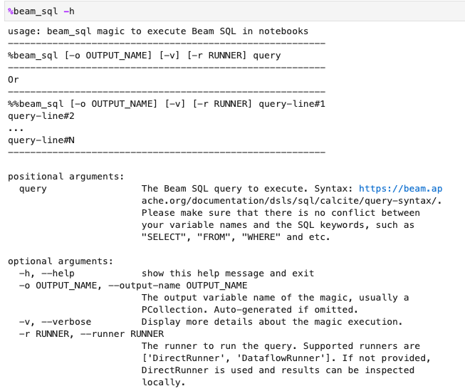
You can check the beam_sql magic usage with the -h or --help option:

You can create a PCollection from constant values:

You can join multiple PCollections:

You can launch a Dataflow job with the -r DataflowRunner or --runner DataflowRunner option:

To learn more, see the example notebook Apache Beam SQL in notebooks.

Accelerate using JIT compiler and GPU

You can use libraries such as numba and GPUs to accelerate your Python code and Apache Beam pipelines. In the Apache Beam notebook instance created with an nvidia-tesla-t4 GPU, to run on GPUs, compile your Python code with numba.cuda.jit. Optionally, to speed up the execution on CPUs, compile your Python code into machine code with numba.jit or numba.njit.

The following example creates a DoFn that processes on GPUs:

class Sampler(beam.DoFn):
    def __init__(self, blocks=80, threads_per_block=64):
        # Uses only 1 cuda grid with below config.
        self.blocks = blocks
        self.threads_per_block = threads_per_block

    def setup(self):
        import numpy as np
        # An array on host as the prototype of arrays on GPU to
        # hold accumulated sub count of points in the circle.
        self.h_acc = np.zeros(
            self.threads_per_block * self.blocks, dtype=np.float32)

    def process(self, element: Tuple[int, int]):
        from numba import cuda
        from numba.cuda.random import create_xoroshiro128p_states
        from numba.cuda.random import xoroshiro128p_uniform_float32

        @cuda.jit
        def gpu_monte_carlo_pi_sampler(rng_states, sub_sample_size, acc):
            """Uses GPU to sample random values and accumulates the sub count
            of values within a circle of radius 1.
            """
            pos = cuda.grid(1)
            if pos < acc.shape[0]:
                sub_acc = 0
                for i in range(sub_sample_size):
                    x = xoroshiro128p_uniform_float32(rng_states, pos)
                    y = xoroshiro128p_uniform_float32(rng_states, pos)
                    if (x * x + y * y) <= 1.0:
                        sub_acc += 1
                acc[pos] = sub_acc

        rng_seed, sample_size = element
        d_acc = cuda.to_device(self.h_acc)
        sample_size_per_thread = sample_size // self.h_acc.shape[0]
        rng_states = create_xoroshiro128p_states(self.h_acc.shape[0], seed=rng_seed)
        gpu_monte_carlo_pi_sampler[self.blocks, self.threads_per_block](
            rng_states, sample_size_per_thread, d_acc)
        yield d_acc.copy_to_host()

The following image demonstrates the notebook running on a GPU:

More details can be found in the example notebook Use GPUs with Apache Beam.

Build a custom container

In most cases, if your pipeline doesn't require additional Python dependencies or executables, Apache Beam can automatically use its official container images to run your user-defined code. These images come with many common Python modules, and you don't have to build or explicitly specify them.

In some cases, you might have extra Python dependencies or even non-Python dependencies. In these scenarios, you can build a custom container and make it available to the Flink cluster to run. The following list provides the advantages of using a custom container:

• Faster setup time for consecutive and interactive executions
• Stable configurations and dependencies
• More flexibility: you can set up more than Python dependencies

The container build process might be tedious, but you can do everything in the notebook using the following usage pattern.

Create a local workspace

First, create a local work directory under the Jupyter home directory.

!mkdir -p /home/jupyter/.flink

Prepare Python dependencies

Next, install all the extra Python dependencies that you might use, and export them into a requirements file.

%pip install dep_a
%pip install dep_b
...

You can explicitly create a requirements file by using the %%writefile notebook magic.

%%writefile /home/jupyter/.flink/requirements.txt
dep_a
dep_b
...

Alternatively, you can freeze all local dependencies into a requirements file. This option might introduce unintended dependencies.

%pip freeze > /home/jupyter/.flink/requirements.txt

Prepare your non-Python dependencies

Copy all non-Python dependencies into the workspace. If you don't have any non-Python dependencies, skip this step.

!cp /path/to/your-dep /home/jupyter/.flink/your-dep
...

Create a Dockerfile

Create a Dockerfile with the %%writefile notebook magic. For example:

%%writefile /home/jupyter/.flink/Dockerfile
FROM apache/beam_python3.7_sdk:2.40.0

COPY  requirements.txt /tmp/requirements.txt
COPY  your_dep /tmp/your_dep
...

RUN python -m pip install -r /tmp/requirements.txt

The example container uses the image of the Apache Beam SDK version 2.40.0 with Python 3.7 as the base, adds a your_dep file, and installs the extra Python dependencies. Use this Dockerfile as a template, and edit it for your use case.

In your Apache Beam pipelines, when referring to non-Python dependencies, use their COPY destinations. For example, /tmp/your_dep is the file path of the your_dep file.

Build a container image in Artifact Registry by using Cloud Build

1. Enable the Cloud Build and Artifact Registry services, if not already enabled.

   !gcloud services enable cloudbuild.googleapis.com
   !gcloud services enable artifactregistry.googleapis.com
   

2. Create an Artifact Registry repository so that you can upload artifacts. Each repository can contain artifacts for a single supported format.

   All repository content is encrypted using either Google-managed or customer-managed encryption keys. Artifact Registry uses Google-managed encryption keys by default and no configuration is required for this option.

   You must have at least Artifact Registry Writer access to the repository.

   Run the following command to create a new repository. The command uses the --async flag and returns immediately, without waiting for the operation in progress to complete.

   gcloud artifacts repositories create REPOSITORY \
   --repository-format=docker \
   --location=LOCATION \
   --async
   

   Replace the following values:

   • REPOSITORY: a name for your repository. For each repository location in a project, repository names must be unique.
   • LOCATION: the location for your repository.

3. Before you can push or pull images, configure Docker to authenticate requests for Artifact Registry. To set up authentication to Docker repositories, run the following command:

   gcloud auth configure-docker LOCATION-docker.pkg.dev
   

   The command updates your Docker configuration. You can now connect with Artifact Registry in your Google Cloud project to push images.

4. Use Cloud Build to build the container image, and save it to Artifact Registry.

   !cd /home/jupyter/.flink \
   && gcloud builds submit \
    --tag LOCATION.pkg.dev/PROJECT_ID/REPOSITORY/flink:latest \
    --timeout=20m
   

   Replace PROJECT_ID with the project ID of your project.

Warning: Don't build the container image on the notebook instance itself, because it isn't a consistent build environment.

Use custom containers

Depending on the runner, you can use custom containers for different purposes.

For general Apache Beam container usage, see:

• Container environments
• Managing Python Pipeline Dependencies

For Dataflow container usage, see:

• Use custom containers in Dataflow

Disable external IP addresses

When creating an Apache Beam notebook instance, to increase security, disable external IP addresses. Because notebook instances need to download some public internet resources, such as Artifact Registry, you need to first create a new VPC network without an external IP address. Then, create a Cloud NAT gateway for this VPC network. For more information about Cloud NAT, see the Cloud NAT documentation. Use the VPC network and Cloud NAT gateway to access the necessary public internet resources without enabling external IP addresses.