This document describes how you query, view, and analyze log entries by using the Google Cloud console. There are two interfaces available to you, the Logs Explorer and Log Analytics. You can query, view, and analyze logs with both interfaces; however, they use different query languages and they have different capabilities. For troubleshooting and exploration of log data, we recommend using the Logs Explorer. To generate insights and trends, we recommend that you use Log Analytics. You can query your logs and save your queries by issuing Logging API commands. You can also query your logs by using Google Cloud CLI.
Logs Explorer
The Logs Explorer is designed to help you troubleshoot and analyze the performance of your services and applications. For example, a histogram displays the rate of errors. If you see a spike in errors or something that is interesting, you can locate and view the corresponding log entries. When a log entry is associated with an error group, the log entry is annotated with a menu of options that let you access more information about the error group.
The same query language is supported by the Cloud Logging API, the Google Cloud CLI, and the Logs Explorer. To simplify query construction when you are using the Logs Explorer, you can build queries by using menus, by entering text, and, in some cases, by using options included with the display of an individual log entry.
The Logs Explorer doesn't support aggregate operations, like counting the number of log entries that contain a specific pattern. To perform aggregate operations, enable analytics on the log bucket and then use Log Analytics.
For details about searching and viewing logs with the Logs Explorer, see View logs by using the Logs Explorer.
Log Analytics
Using Log Analytics, you can run queries that analyze your log data, and then you can view or chart the query results. Charts let you identify patterns and trends in your logs over time. The following screenshot illustrates the charting capabilities in Log Analytics:
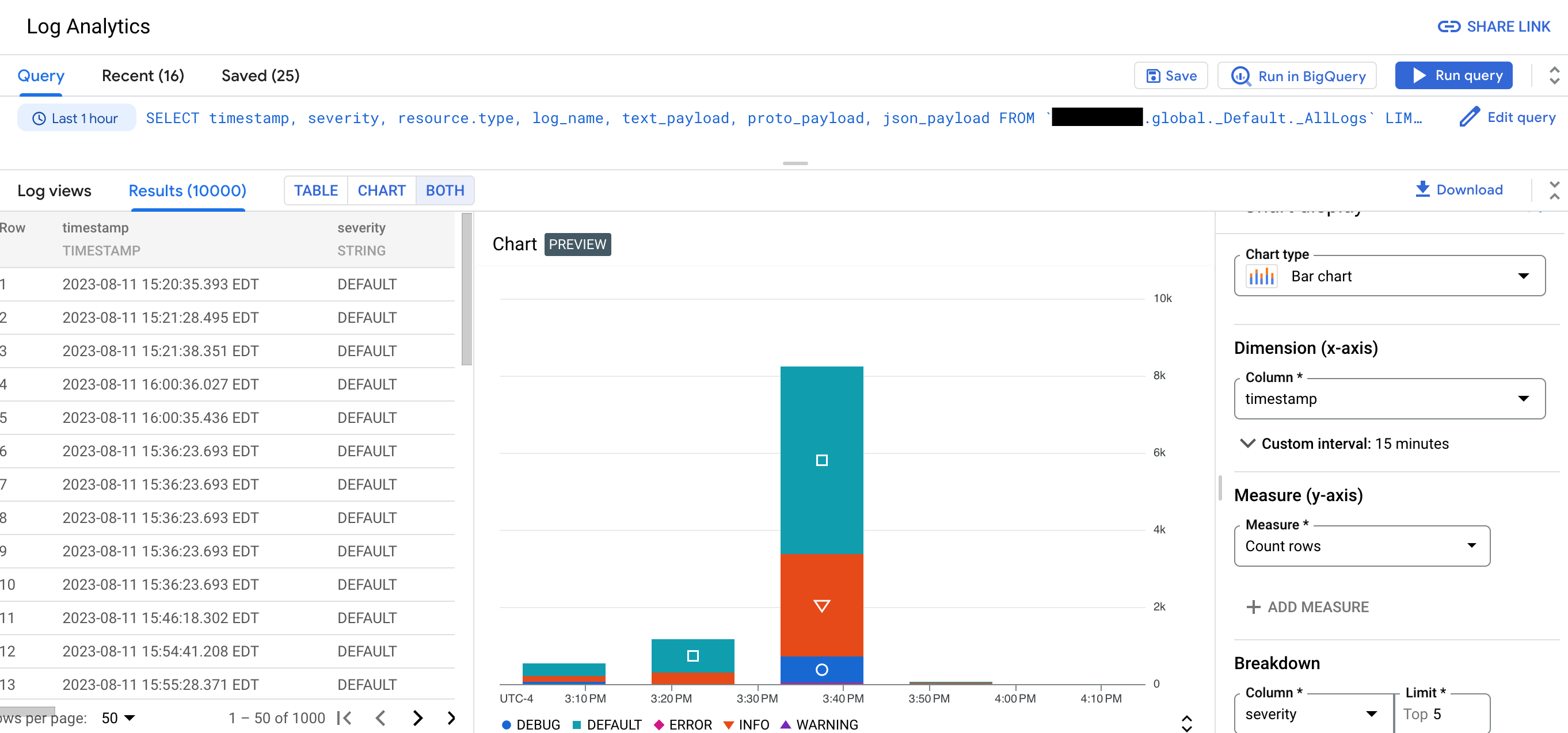
For example, suppose that you are troubleshooting a problem and you want to know the average latency for HTTP requests issued to a specific URL over time. When a log bucket is upgraded to use Log Analytics, you can write a SQL query or use the query builder to query logs stored in your log bucket.
These SQL queries can also include pipe syntax. By grouping and aggregating your logs, you can gain insights into your log data which can help you reduce time spent troubleshooting.
Log Analytics lets you query
log views or an
analytics view. Log views have a fixed schema which
corresponds to the LogEntry data structure.
Because the creator of an analytics view determines the schema, one use
case for analytics views is to transform log data from the
LogEntry format into a format that is more suitable for you.
You can also use BigQuery to query your data. For example, suppose that you want to use BigQuery to compare URLs in your logs with a public dataset of known malicious URLs. To make your log data visible to BigQuery, upgrade your bucket to use Log Analytics and then create a linked dataset.
You can continue to troubleshoot issues and view individual log entries in upgraded log buckets by using the Logs Explorer.
Restrictions
To upgrade an existing log bucket to use Log Analytics, the following restrictions apply:
- The log bucket was created at the Google Cloud project level.
- The log bucket is unlocked unless it is the
_Requiredbucket. - There aren't pending updates to the bucket.
Log entries written before a bucket is upgraded aren't immediately available. However, when the backfill operation completes, you can analyze these log entries. The backfill process might take several days.
You can't use the Log Analytics page to query log views when the log bucket has field-level access controls configured. However, you can issue queries through the Logs Explorer page, and you can query a linked BigQuery dataset. Because BigQuery doesn't honor field-level access controls, if you query a linked dataset, then you can query all fields in the log entries.
If you query multiple log views, then they must be stored in the same location. For example, if two views are located in the
us-east1location, then one query can query both views. You can also query two views that are located in theusmulti-region. However, if a view's location isglobal, then that view can reside in any physical location. Therefore, joins between two views that have the location ofglobalmight fail.If you query multiple log views and their underlying log buckets are configured with different Cloud KMS keys, then the query fails unless the following constraints are met:
- A folder or organization that is a parent resource of the log buckets is configured with a default key.
- The default key is in the same location as the log buckets.
When the previous constraints are satisfied, the parent's Cloud KMS key encrypts any temporary data generated by a Log Analytics query.
Duplicate log entries aren't removed before a query is run. This behavior is different than when you query log entries by using the Logs Explorer, which removes duplicate entries by comparing the log names, timestamps, and insert ID fields. For more information, see Troubleshoot: There are duplicate log entries in my Log Analytics results.
Pricing
For pricing information, see Google Cloud Observability pricing page. If you route log data to other Google Cloud services, then see the following documents:
There are no BigQuery ingestion or storage costs when you upgrade a bucket to use Log Analytics and then create a linked dataset. When you create a linked dataset for a log bucket, you don't ingest your log data into BigQuery. Instead, you get read access to the log data stored in your log bucket through the linked dataset.
BigQuery analysis charges apply when you run SQL queries on BigQuery linked datasets, which includes using the BigQuery Studio page, the BigQuery API, and the BigQuery command-line tool.
Blogs
For more information about Log Analytics, see the following blog posts:
- For an overview of Log Analytics, see Log Analytics in Cloud Logging is now GA.
- To learn about creating charts generated by Log Analytics queries and saving those charts to custom dashboards, see Announcing Log Analytics charts and dashboards in Cloud Logging in public preview.
- To learn about analyzing audit logs by using Log Analytics, see Gleaning security insights from audit logs with Log Analytics.
- If you route logs to BigQuery and want to understand the difference between that solution and using Log Analytics, then see Moving to Log Analytics for BigQuery export users.
What's next
- Create a log bucket and upgrade it to use Log Analytics
- Upgrade an existing bucket to use Log Analytics
Query and view logs:
Sample queries: