Use the Apache Beam interactive runner with JupyterLab notebooks to complete the following tasks:
- Iteratively develop pipelines.
- Inspect your pipeline graph.
- Parse individual
PCollectionsin a read-eval-print-loop (REPL) workflow.
These Apache Beam notebooks are made available through Vertex AI Workbench, a service that hosts notebook virtual machines pre-installed with the latest data science and machine learning frameworks. Dataflow only supports Workbench instances that use the Apache Beam container.
This guide focuses on the features introduced by Apache Beam notebooks, but doesn't show how to build a notebook. For more information about Apache Beam, see the Apache Beam programming guide.
Support and limitations
- Apache Beam notebooks only support Python.
- Apache Beam pipeline segments running in these notebooks are run in a test environment, and not against a production Apache Beam runner. To launch the notebooks on the Dataflow service, export the pipelines created in your Apache Beam notebook. For more details, see Launch Dataflow jobs from a pipeline created in your notebook.
Before you begin
- Sign in to your Google Cloud Platform account. If you're new to Google Cloud, create an account to evaluate how our products perform in real-world scenarios. New customers also get $300 in free credits to run, test, and deploy workloads.
-
In the Google Cloud console, on the project selector page, select or create a Google Cloud project.
Roles required to select or create a project
- Select a project: Selecting a project doesn't require a specific IAM role—you can select any project that you've been granted a role on.
-
Create a project: To create a project, you need the Project Creator
(
roles/resourcemanager.projectCreator), which contains theresourcemanager.projects.createpermission. Learn how to grant roles.
-
Verify that billing is enabled for your Google Cloud project.
-
Enable the Compute Engine and Notebooks APIs.
Roles required to enable APIs
To enable APIs, you need the Service Usage Admin IAM role (
roles/serviceusage.serviceUsageAdmin), which contains theserviceusage.services.enablepermission. Learn how to grant roles. -
In the Google Cloud console, on the project selector page, select or create a Google Cloud project.
Roles required to select or create a project
- Select a project: Selecting a project doesn't require a specific IAM role—you can select any project that you've been granted a role on.
-
Create a project: To create a project, you need the Project Creator
(
roles/resourcemanager.projectCreator), which contains theresourcemanager.projects.createpermission. Learn how to grant roles.
-
Verify that billing is enabled for your Google Cloud project.
-
Enable the Compute Engine and Notebooks APIs.
Roles required to enable APIs
To enable APIs, you need the Service Usage Admin IAM role (
roles/serviceusage.serviceUsageAdmin), which contains theserviceusage.services.enablepermission. Learn how to grant roles.
Before creating your Apache Beam notebook instance, enable additional APIs for pipelines that use other services, such as Pub/Sub.
If not specified, the notebook instance is executed by the default Compute Engine service account with the IAM project editor role. If the project explicitly limits the roles of the service account, make sure it still has enough authorization to run your notebooks. For example, reading from a Pub/Sub topic implicitly creates a subscription, and your service account needs an IAM Pub/Sub editor role. By contrast, reading from a Pub/Sub subscription only requires an IAM Pub/Sub subscriber role.
When you finish this guide, to avoid continued billing, delete the resources you created. For more details, see Cleaning up.
Launch an Apache Beam notebook instance
In the Google Cloud console, go to the Dataflow Workbench page.
Make sure that you're on the INSTANCES tab.
In the toolbar, click Create new.
In the Environment section, for Environment, Container should be Apache Beam. Only JupyterLab 3.x is supported for Apache Beam notebooks.
Optional: If you want to run notebooks on a GPU, in the Machine type section, select a machine type that supports GPUs. For more information, see GPU platforms.
In the Networking section, select a subnetwork for the notebook VM.
Optional: If you want to set up a custom notebook instance, see Create an instance using a custom container.
Click Create. Dataflow Workbench creates a new Apache Beam notebook instance.
After the notebook instance is created, the Open JupyterLab link becomes active. Click Open JupyterLab.
Optional: Install dependencies
Apache Beam notebooks already come with Apache Beam and
Google Cloud connector dependencies installed. If your pipeline contains
custom connectors or custom PTransforms that depend on third-party libraries,
install them after you create a notebook instance.
Example Apache Beam notebooks
After you create a notebook instance, open it in JupyterLab. In the Files tab in the JupyterLab sidebar, the Examples folder contains example notebooks. For more information about working with JupyterLab files, see Working with files in the JupyterLab user guide.
The following notebooks are available:
- Word Count
- Streaming Word Count
- Streaming NYC Taxi Ride Data
- Apache Beam SQL in notebooks with comparisons to pipelines
- Apache Beam SQL in notebooks with the Dataflow Runner
- Apache Beam SQL in notebooks
- Dataflow Word Count
- Interactive Flink at Scale
- RunInference
- Use GPUs with Apache Beam
- Visualize Data
The Tutorials folder contains additional tutorials that explain the fundamentals of Apache Beam. The following tutorials are available:
- Basic Operations
- Element Wise Operations
- Aggregations
- Windows
- I/O Operations
- Streaming
- Final Exercises
These notebooks include explanatory text and commented code blocks to help you understand Apache Beam concepts and API usage. The tutorials also provide exercises for you to practice concepts.
The following sections use example code from the Streaming Word Count notebook. The code snippets in this guide and what is found in the Streaming Word Count notebook might have minor discrepancies.
Create a notebook instance
Navigate to File > New > Notebook and select a kernel that is Apache Beam 2.22 or later.
Apache Beam notebooks are built against the master branch of the Apache Beam SDK. This means that the latest version of the kernel shown in the notebooks UI might be ahead of the most recently released version of the SDK.
Apache Beam is installed on your notebook instance, so include the interactive_runner and interactive_beam modules in your notebook.
import apache_beam as beam
from apache_beam.runners.interactive.interactive_runner import InteractiveRunner
import apache_beam.runners.interactive.interactive_beam as ib
If your notebook uses other Google APIs, add the following import statements:
from apache_beam.options import pipeline_options
from apache_beam.options.pipeline_options import GoogleCloudOptions
import google.auth
Set interactivity options
The following line sets the amount of time the InteractiveRunner records data from an unbounded source. In this example, the duration is set to 10 minutes.
ib.options.recording_duration = '10m'
You can also change the recording size limit (in bytes) for an unbounded source
by using the recording_size_limit property.
# Set the recording size limit to 1 GB.
ib.options.recording_size_limit = 1e9
For additional interactive options, see the interactive_beam.options class.
Create your pipeline
Initialize the pipeline using an InteractiveRunner object.
options = pipeline_options.PipelineOptions(flags={})

# Set the pipeline mode to stream the data from Pub/Sub.
options.view_as(pipeline_options.StandardOptions).streaming = True

# Set the project to the default project in your current Google Cloud Platform environment.
# The project is used to create a subscription to the Pub/Sub topic.
_, options.view_as(GoogleCloudOptions).project = google.auth.default()

p = beam.Pipeline(InteractiveRunner(), options=options)
Read and visualize the data
The following example shows an Apache Beam pipeline that creates a subscription to the given Pub/Sub topic and reads from the subscription.
words = p | "read" >> beam.io.ReadFromPubSub(topic="projects/pubsub-public-data/topics/shakespeare-kinglear")
The pipeline counts the words by windows from the source. It creates fixed windowing with each window being 10 seconds in duration.
windowed_words = (words
   | "window" >> beam.WindowInto(beam.window.FixedWindows(10)))
After the data is windowed, the words are counted by window.
windowed_word_counts = (windowed_words
   | "count" >> beam.combiners.Count.PerElement())
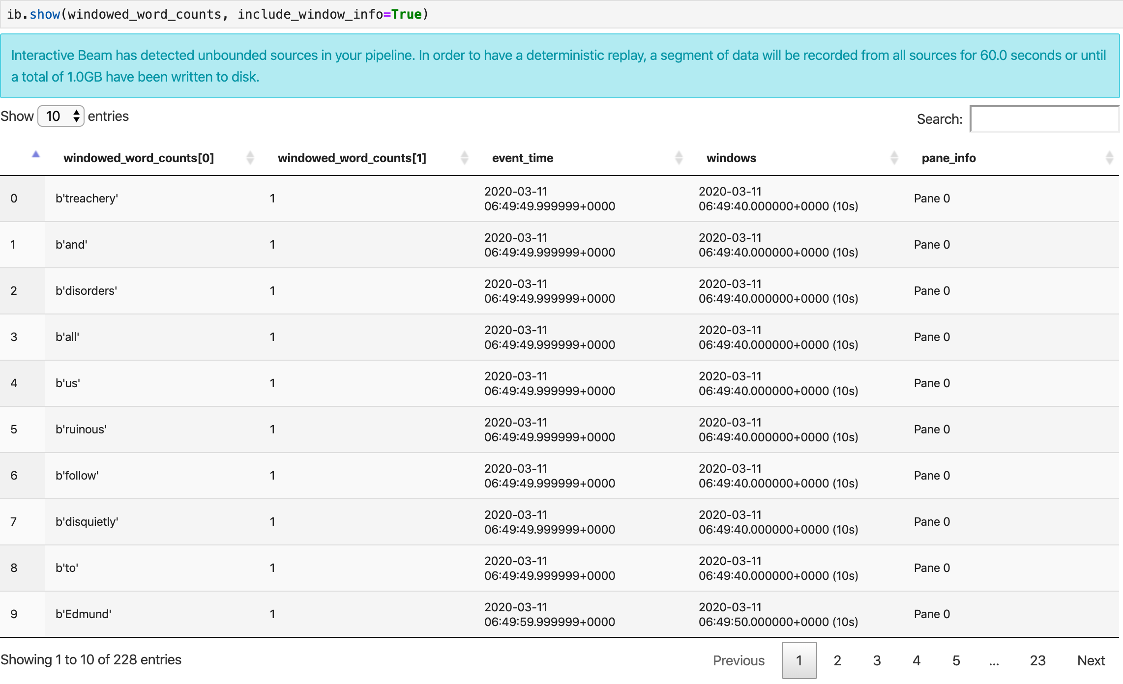
The show() method visualizes the resulting PCollection in the notebook.
ib.show(windowed_word_counts, include_window_info=True)
You can scope the result set back from show() by setting two optional
parameters: n and duration.
- Set
nto limit the result set to show at mostnnumber of elements, such as 20. Ifnis not set, the default behavior is to list the most recent elements captured until the source recording is over. - Set
durationto limit the result set to a specified number of seconds worth of data starting from the beginning of the source recording. Ifdurationisn't set, the default behavior is to list all elements until the recording is over.
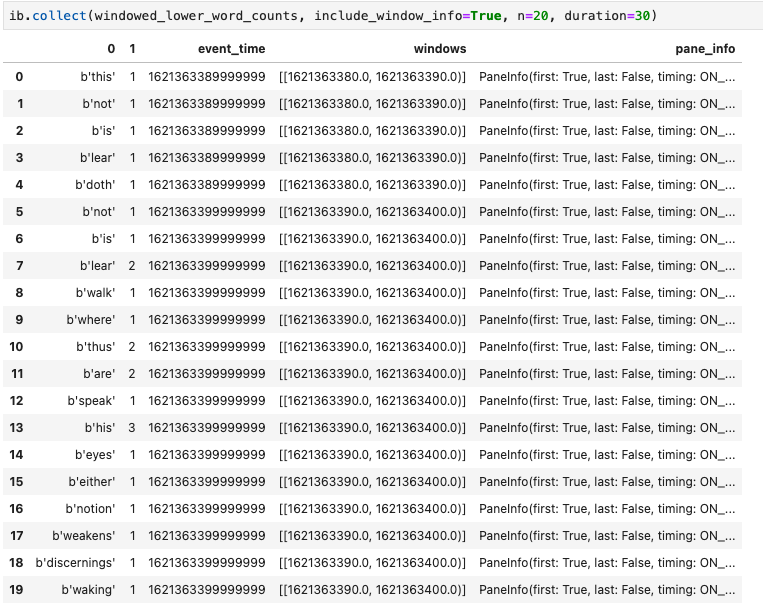
If both optional parameters are set, show() stops whenever either threshold is met. In the following example, show() returns at most 20 elements that are computed based on the first 30 seconds worth of data from the recorded sources.
ib.show(windowed_word_counts, include_window_info=True, n=20, duration=30)
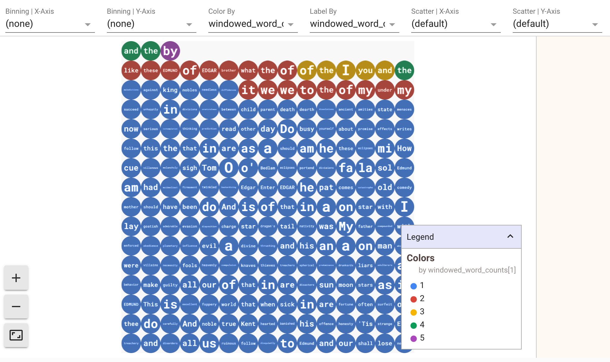
To display visualizations of your data, pass visualize_data=True into the
show() method. You can apply multiple filters to your visualizations. The
following visualization allows you to filter by label and axis:
To ensure replayability while prototyping streaming pipelines, the
show() method calls reuse the captured data by default. To change this
behavior and have the show() method always fetch new data, set
interactive_beam.options.enable_capture_replay = False. Also, if you add a
second unbounded source to your notebook, the data from the previous unbounded
source is discarded.
Another useful visualization in Apache Beam notebooks is a Pandas DataFrame. The following example first converts the words to lowercase and then computes the frequency of each word.
windowed_lower_word_counts = (windowed_words
   | beam.Map(lambda word: word.lower())
   | "count" >> beam.combiners.Count.PerElement())
The collect() method provides the output in a Pandas DataFrame.
ib.collect(windowed_lower_word_counts, include_window_info=True)
Editing and rerunning a cell is a common practice in notebook
development. When you edit and rerun a cell in a Apache Beam notebook,
the cell doesn't undo the intended action of the code in the original cell. For
example, if a cell adds a PTransform to a pipeline, rerunning that cell
adds an additional PTransform to the pipeline. If you want to clear the state,
restart the kernel, and then rerun the cells.
Visualize the data through the Interactive Beam inspector
You might find it distracting to introspect the data of a PCollection by
constantly calling show() and collect(), especially when the output takes up
a lot of the space on your screen and makes it hard to navigate through the
notebook. You might also want to compare multiple PCollections side by side to
validate if a transform works as intended. For example, when one PCollection
goes through a transform and produces the other. For these use cases, the
Interactive Beam inspector is a convenient solution.
Interactive Beam inspector is provided as a JupyterLab extension
apache-beam-jupyterlab-sidepanel
preinstalled in the Apache Beam notebook. With the extension,
you can interactively inspect the state of pipelines and data associated with
each PCollection without explicitly invoking show() or collect().
There are 3 ways to open the inspector:
Click
Interactive Beamon the top menu bar of JupyterLab. In the dropdown, locateOpen Inspector, and click it to open the inspector.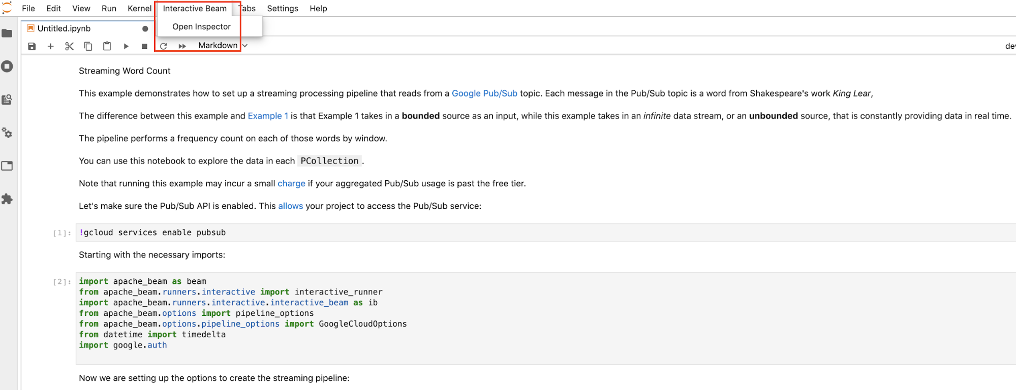
Use the launcher page. If there is no launcher page opened, click
File->New Launcherto open it. On the launcher page, locateInteractive Beamand clickOpen Inspectorto open the inspector.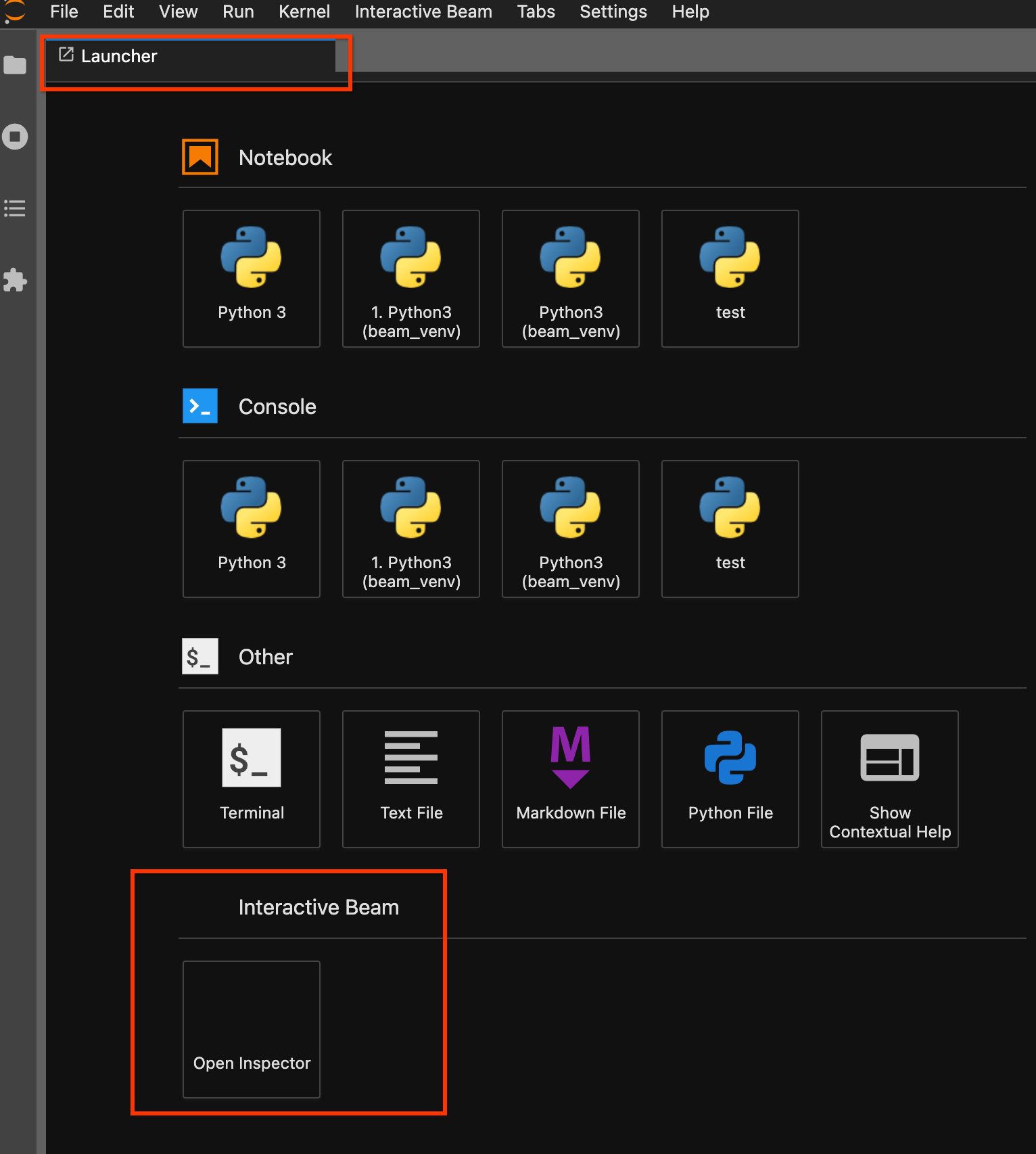
Use the command palette. On the JupyterLab menu bar, click
View>Activate Command Palette. In the dialog, search forInteractive Beamto list all options of the extension. ClickOpen Inspectorto open the inspector.
When the inspector is about to open:
If there is exactly one notebook open, the inspector automatically connects to it.
If no notebook is open, a dialog appears that lets you select a kernel.
If multiple notebooks are open, a dialog appears that lets you select the notebook session.
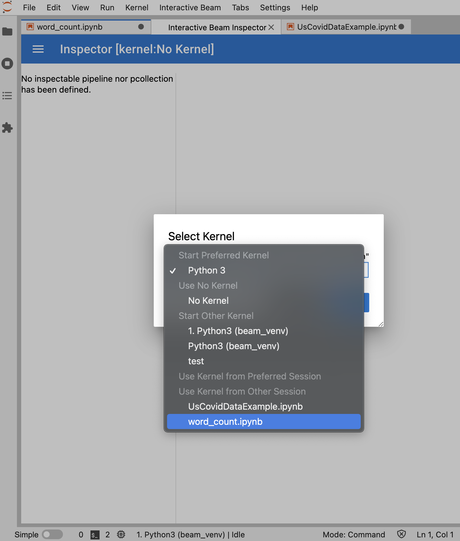
It's recommended to open at least one notebook and select a kernel for it
before opening the inspector. If you open an inspector with a kernel before
opening any notebook, later when you open a notebook to connect to the
inspector, you have to select the Interactive Beam Inspector Session from Use
Kernel from Preferred Session. An inspector and a notebook are connected when
they share the same session, not different sessions created from the same
kernel. Selecting the same kernel from Start Preferred Kernel creates a
new session that is independent from existing sessions of opened notebooks or
inspectors.
You can open multiple inspectors for an opened notebook and arrange the inspectors by dragging and dropping their tabs freely in the workspace.
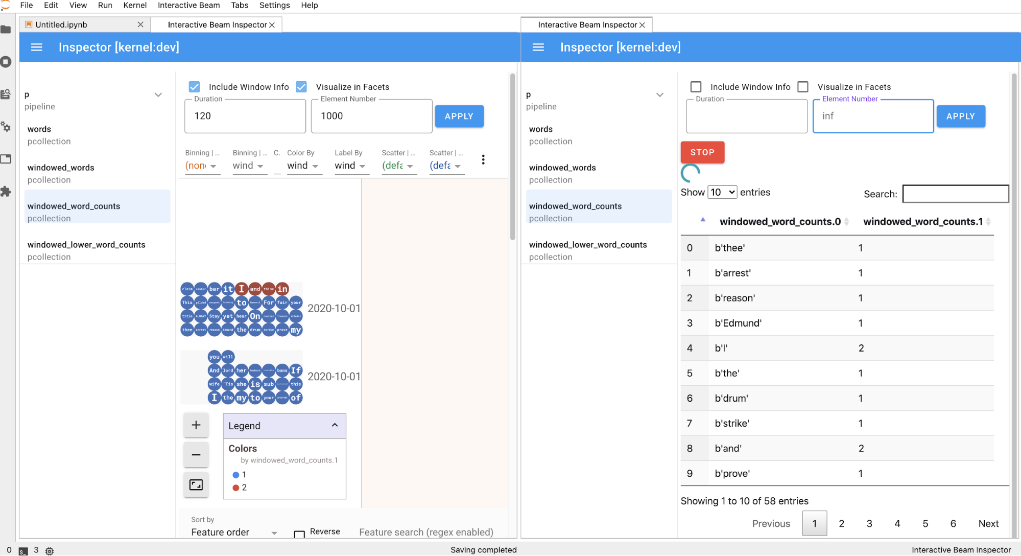
The inspector page automatically refreshes when you run cells in the
notebook. The page lists pipelines and PCollections defined in the
connected notebook. PCollections are organized by the pipelines they belong
to, and you can collapse them by clicking the header pipeline.
For the items in the pipelines and PCollections list, on click, the inspector
renders corresponding visualizations on the right side:
If it's a
PCollection, the inspector renders its data (dynamically if the data is still coming in for unboundedPCollections) with additional widgets to tune the visualization after clicking theAPPLYbutton.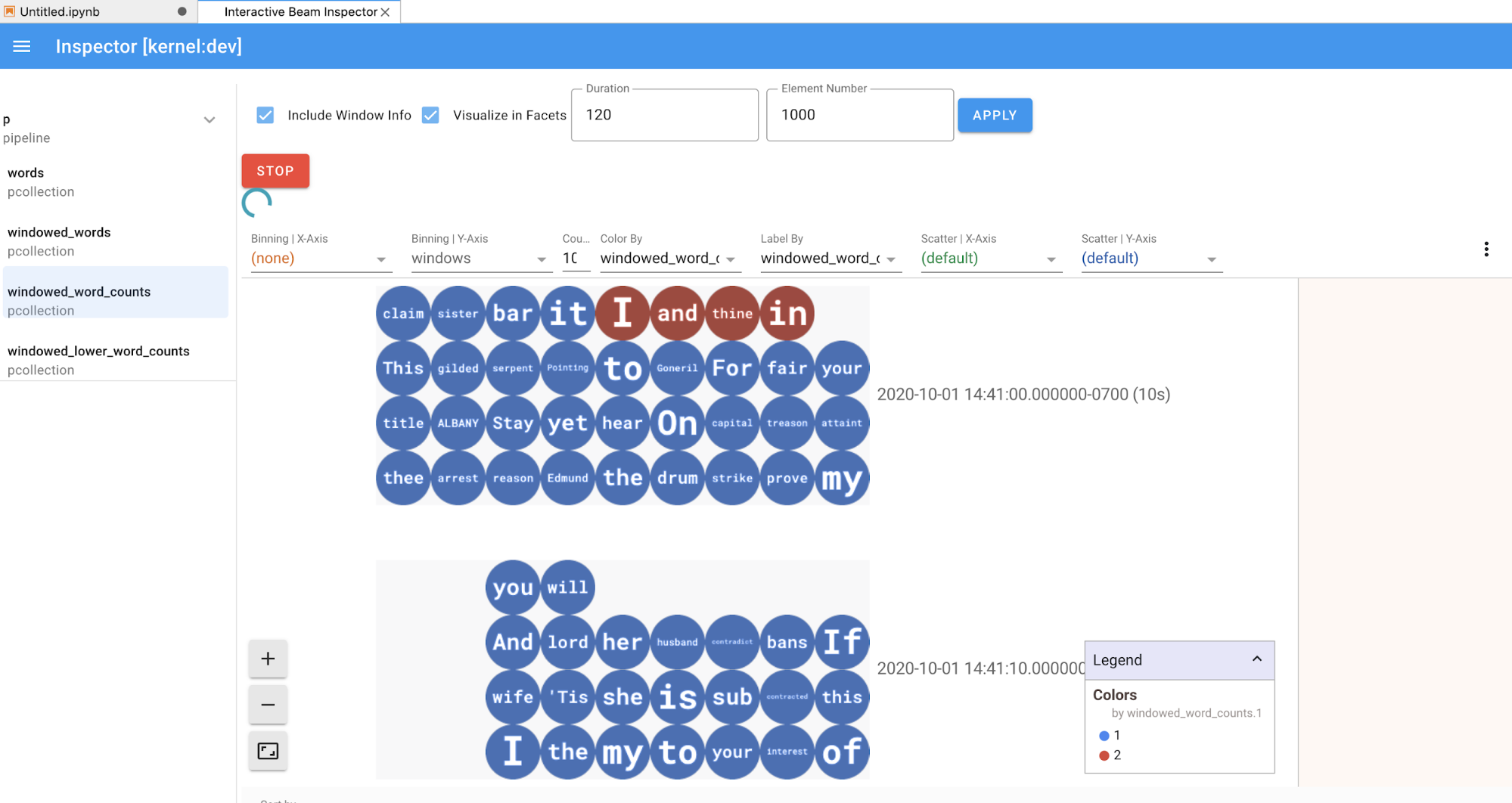
Because the inspector and the opened notebook share the same kernel session, they block each other from running. For example, if the notebook is busy running code, the inspector does not update until the notebook completes that execution. Conversely, if you want to run code immediately in your notebook while the inspector is visualizing a
PCollectiondynamically, you have to click theSTOPbutton to stop the visualization and preemptively release the kernel to the notebook.If it's a pipeline, the inspector displays the pipeline graph.
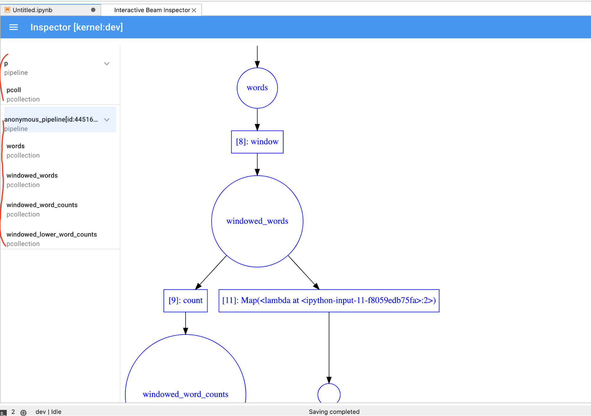
You might notice anonymous pipelines. Those pipelines have
PCollections that you can access, but they are no longer referenced by the main
session. For example:
p = beam.Pipeline()
pcoll = p | beam.Create([1, 2, 3])

p = beam.Pipeline()
The previous example creates an empty pipeline p and an anonymous pipeline that
contains one PCollection pcoll. You can access the anonymous pipeline
by using pcoll.pipeline.
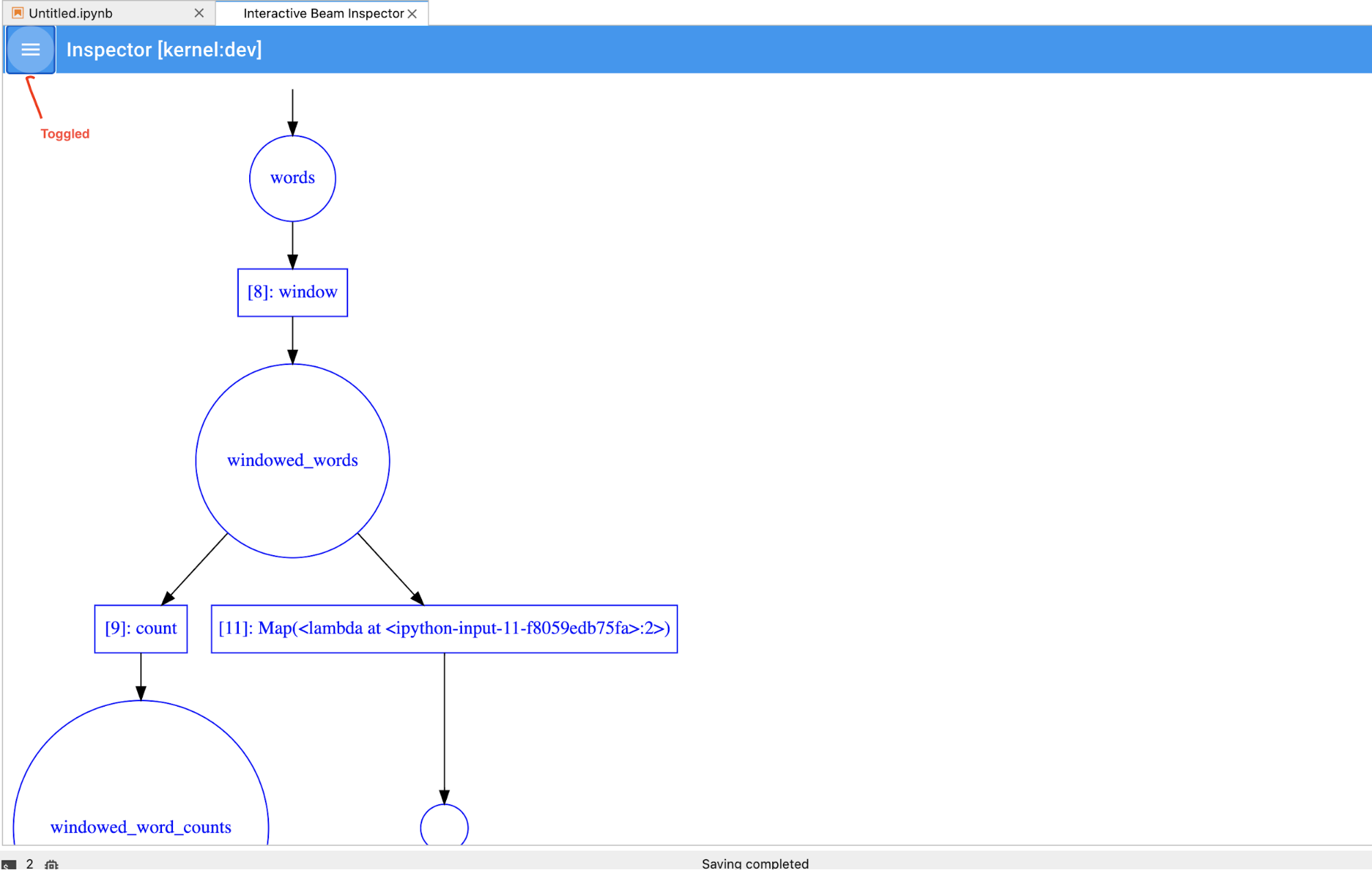
You can toggle the pipeline and PCollection list to save space for
big visualizations.
Understand a pipeline's recording status
In addition to visualizations, you can also inspect the recording status for one or all pipelines in your notebook instance by calling describe.
# Return the recording status of a specific pipeline. Leave the parameter list empty to return
# the recording status of all pipelines.
ib.recordings.describe(p)
The describe() method provides the following details:
- Total size (in bytes) of all of the recordings for the pipeline on disk
- Start time of when the background recording job started (in seconds from Unix epoch)
- Current pipeline status of the background recording job
- Python variable for the pipeline
Launch Dataflow jobs from a pipeline created in your notebook
- Optional: Before using your notebook to run Dataflow jobs, restart the kernel, rerun all cells, and verify the output. If you skip this step, hidden states in the notebook might affect the job graph in the pipeline object.
- Enable the Dataflow API.
Add the following import statement:
from apache_beam.runners import DataflowRunnerPass in your pipeline options.
# Set up Apache Beam pipeline options.
options = pipeline_options.PipelineOptions()

# Set the project to the default project in your current Google Cloud
# environment.
_, options.view_as(GoogleCloudOptions).project = google.auth.default()

# Set the Google Cloud region to run Dataflow.
options.view_as(GoogleCloudOptions).region = 'us-central1'

# Choose a Cloud Storage location.
dataflow_gcs_location = 'gs://<change me>/dataflow'

# Set the staging location. This location is used to stage the
# Dataflow pipeline and SDK binary.
options.view_as(GoogleCloudOptions).staging_location = '%s/staging' % dataflow_gcs_location

# Set the temporary location. This location is used to store temporary files
# or intermediate results before outputting to the sink.
options.view_as(GoogleCloudOptions).temp_location = '%s/temp' % dataflow_gcs_location

# If and only if you are using Apache Beam SDK built from source code, set
# the SDK location. This is used by Dataflow to locate the SDK
# needed to run the pipeline.
options.view_as(pipeline_options.SetupOptions).sdk_location = (
    '/root/apache-beam-custom/packages/beam/sdks/python/dist/apache-beam-%s0.tar.gz' %
    beam.version.__version__)
You can adjust the parameter values. For example, you can change the
regionvalue fromus-central1.Run the pipeline with
DataflowRunner. This step runs your job on the Dataflow service.runner = DataflowRunner() runner.run_pipeline(p, options=options)pis a pipeline object from Creating your pipeline.
For an example about how to perform this conversion on an interactive notebook, see the Dataflow Word Count notebook in your notebook instance.
Alternatively, you can export your notebook as an executable script, modify the
generated .py file using the previous steps, and then deploy your
pipeline to the Dataflow
service.
Save your notebook
Notebooks you create are saved locally in your running notebook instance. If you
reset or
shut down the notebook instance during development, those new notebooks are
persisted as long as they are created under the /home/jupyter directory.
However, if a notebook instance is deleted, those notebooks are also deleted.
To keep your notebooks for future use, download them locally to your workstation, save them to GitHub, or export them to a different file format.
Save your notebook to additional persistent disks
If you want to keep your work such as notebooks and scripts throughout various notebook instances, store them in Persistent Disk.
Create or attach a Persistent Disk. Follow the instructions to use
sshto connect to the VM of the notebook instance and issue commands in the opened Cloud Shell.Note the directory where the Persistent Disk is mounted, for example,
/mnt/myDisk.Edit the VM details of the notebook instance to add an entry to the
Custom
metadata
: key -container-custom-params; value --v /mnt/myDisk:/mnt/myDisk.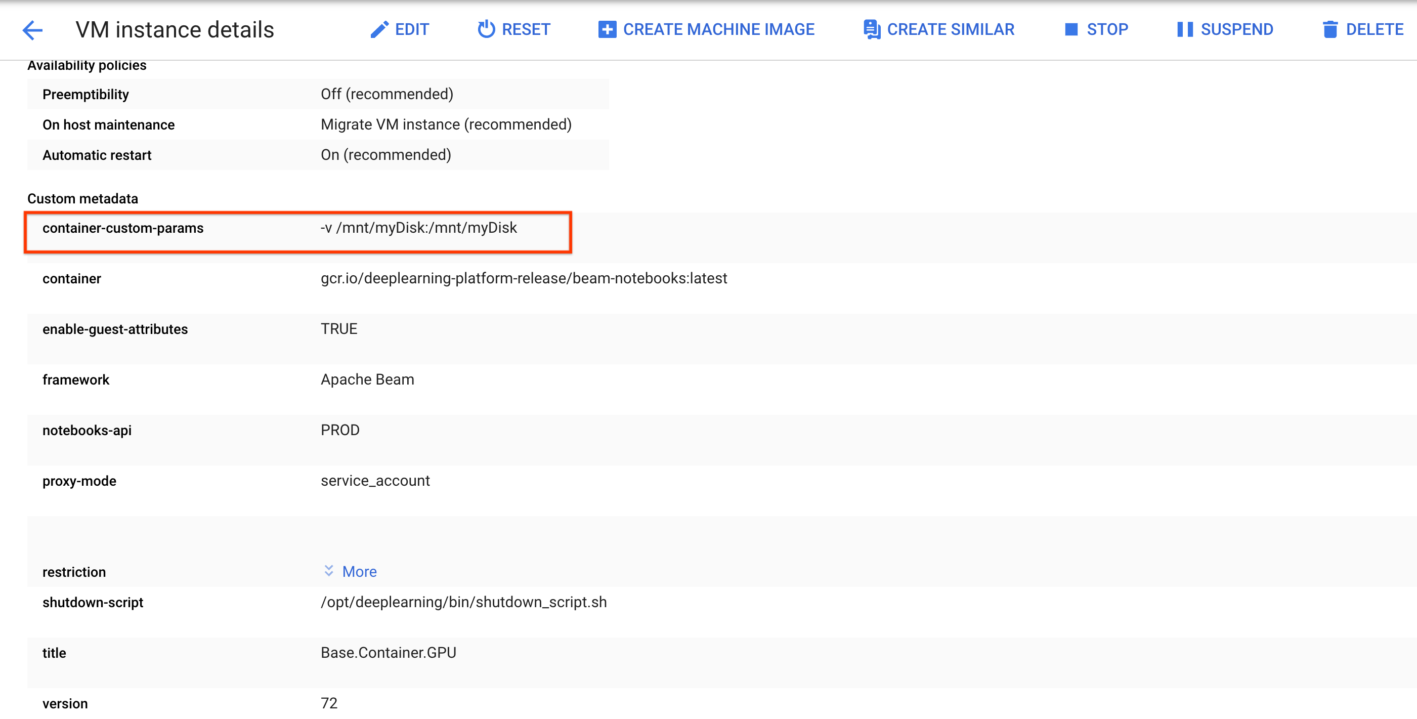
Click Save.
To update these changes, reset the notebook instance.

After the reset, click Open JupyterLab. It might take time for the JupyterLab UI to become available. After the UI appears, open a terminal and run the following command:
ls -al /mntThe/mnt/myDiskdirectory should be listed.
Now you can save your work to the /mnt/myDisk directory. Even if the notebook
instance is deleted, the Persistent Disk exists in your project. You
can then attach this Persistent Disk to other notebook instances.
Clean up
After you finish using your Apache Beam notebook instance, clean up the resources you created on Google Cloud by shutting down the notebook instance.
What's next
- Learn about advanced features that you can use with your Apache Beam notebooks. Advanced features include the following workflows:
