检测数据异常

---

注意：Dataplex Explore 已弃用。对 Explore 的支持将于 2025 年 6 月 30 日结束。我们建议您将资产迁移到 BigQuery Studio，以便在所有 Google Cloud 分析工具中获得简化的数据探索体验。请参阅从“探索”迁移到 BigQuery Studio。

本文档介绍了如何使用 Dataplex Explore 检测零售交易数据集中的异常情况。

借助数据探索工作台（即探索），数据分析师可以实时以交互方式查询和探索大型数据集。“探索”功能可帮助您从数据中获得数据洞见，并让您查询存储在 Cloud Storage 和 BigQuery 中的数据。探索使用无服务器 Spark 平台，因此您无需管理和扩缩底层基础架构。

目标

本教程介绍如何完成以下任务：

• 使用“探索”的 Spark SQL 工作台编写和执行 Spark SQL 查询。
• 使用 JupyterLab 笔记本查看结果。
• 安排笔记本定期执行，以便监控数据是否存在异常。

费用

在本文档中，您将使用 Google Cloud 的以下收费组件：

• Dataplex
• Cloud Storage

您可使用价格计算器根据您的预计使用情况来估算费用。 Google Cloud 新用户可能有资格申请免费试用。

完成本文档中描述的任务后，您可以通过删除所创建的资源来避免继续计费。如需了解详情，请参阅清理。

准备工作

1. Sign in to your Google Cloud account. If you're new to Google Cloud, create an account to evaluate how our products perform in real-world scenarios. New customers also get $300 in free credits to run, test, and deploy workloads.
2. Install the Google Cloud CLI.

3. To initialize the gcloud CLI, run the following command:

   gcloud init

4. Create or select a Google Cloud project.

   Note: If you don't plan to keep the resources that you create in this procedure, create a project instead of selecting an existing project. After you finish these steps, you can delete the project, removing all resources associated with the project.

   • Create a Google Cloud project:

     gcloud projects create PROJECT_ID

     Replace PROJECT_ID with a name for the Google Cloud project you are creating.

   • Select the Google Cloud project that you created:

     gcloud config set project PROJECT_ID

     Replace PROJECT_ID with your Google Cloud project name.

5. Make sure that billing is enabled for your Google Cloud project.

6. Install the Google Cloud CLI.

7. To initialize the gcloud CLI, run the following command:

   gcloud init

8. Create or select a Google Cloud project.

   Note: If you don't plan to keep the resources that you create in this procedure, create a project instead of selecting an existing project. After you finish these steps, you can delete the project, removing all resources associated with the project.

   • Create a Google Cloud project:

     gcloud projects create PROJECT_ID

     Replace PROJECT_ID with a name for the Google Cloud project you are creating.

   • Select the Google Cloud project that you created:

     gcloud config set project PROJECT_ID

     Replace PROJECT_ID with your Google Cloud project name.

9. Make sure that billing is enabled for your Google Cloud project.

注意： “探索”功能仅在 us-central1 和 europe-west2 地区提供。 确保您的所有数据源（Cloud Storage 存储分区和 BigQuery 表）都位于同一区域。了解详情。

准备数据以进行探索

1. 下载 Parquet 文件 retail_offline_sales_march。

   下载 Parquet 文件

2. 按照以下步骤创建一个名为 offlinesales_curated 的 Cloud Storage 存储分区：

   1. In the Google Cloud console, go to the Cloud Storage Buckets page.

      Go to Buckets page

   2. Click Create bucket.
   3. On the Create a bucket page, enter your bucket information. To go to the next step, click Continue.
      • For Name your bucket, enter a name that meets the bucket naming requirements.
      • For Choose where to store your data, do the following:
        • Select a Location type option.
        • Select a Location option.
      • For Choose a default storage class for your data, select a storage class.
      • For Choose how to control access to objects, select an Access control option.
      • For Advanced settings (optional), specify an encryption method, a retention policy, or bucket labels.
   4. Click Create.

3. 按照从文件系统上传对象中的步骤，将您下载的 offlinesales_march_parquet 文件上传到您创建的 offlinesales_curated Cloud Storage 存储分区。

4. 按照创建数据湖中的步骤创建一个 Dataplex 数据湖，并将其命名为 operations。

5. 在 operations 数据湖中，按照添加可用区中的步骤添加一个可用区并将其命名为 procurement。

6. 在 procurement 区域中，按照添加资产中的步骤，将您创建的 offlinesales_curated Cloud Storage 存储分区添加为资产。

选择要探索的表

1. 在 Google Cloud 控制台中，前往 Dataplex 的探索页面。

2. 在湖泊字段中，选择 operations 湖泊。

3. 点击 operations 数据湖。

4. 前往 procurement 区域，然后点击表格以浏览其元数据。

   在下图中，所选的采购区域包含一个名为 Offline 的表，其中包含元数据：orderid、product、quantityordered、unitprice、orderdate 和 purchaseaddress。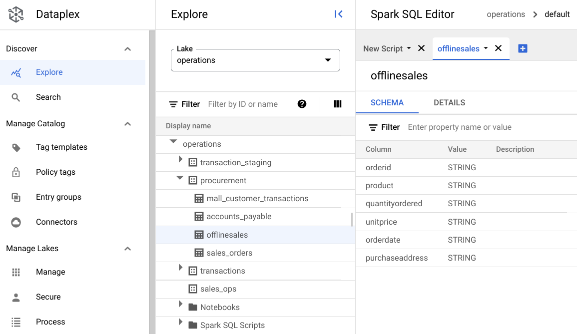

   

5. 在 Spark SQL 编辑器中，点击 Add（添加）。系统会显示一个 Spark SQL 脚本。

6. 可选：在分屏标签页视图中打开脚本，以并排查看元数据和新脚本。在新的脚本标签页中，点击 More（更多），然后选择 Split tab to the right（将标签页拆分到右侧）或 Split tab to the left（将标签页拆分到左侧）。

探索数据

环境可为您的 Spark SQL 查询和笔记本提供无服务器计算资源，以便在数据湖中运行。在编写 Spark SQL 查询之前，请创建一个环境来运行查询。

使用以下 SparkSQL 查询探索数据。在 SparkSQL 编辑器中，将查询输入到新脚本窗格中。

表格中的 10 行示例

1. 输入以下查询：

   select * from procurement.offlinesales where orderid != 'orderid' limit 10;
   

2. 点击运行。

获取数据集中的交易总数

1. 输入以下查询：

   select count(*) from procurement.offlinesales where orderid!='orderid';
   

2. 点击运行。

查找数据集中不同商品类型的数量

1. 输入以下查询：

   select count(distinct product) from procurement.offlinesales where orderid!='orderid';
   

2. 点击运行。

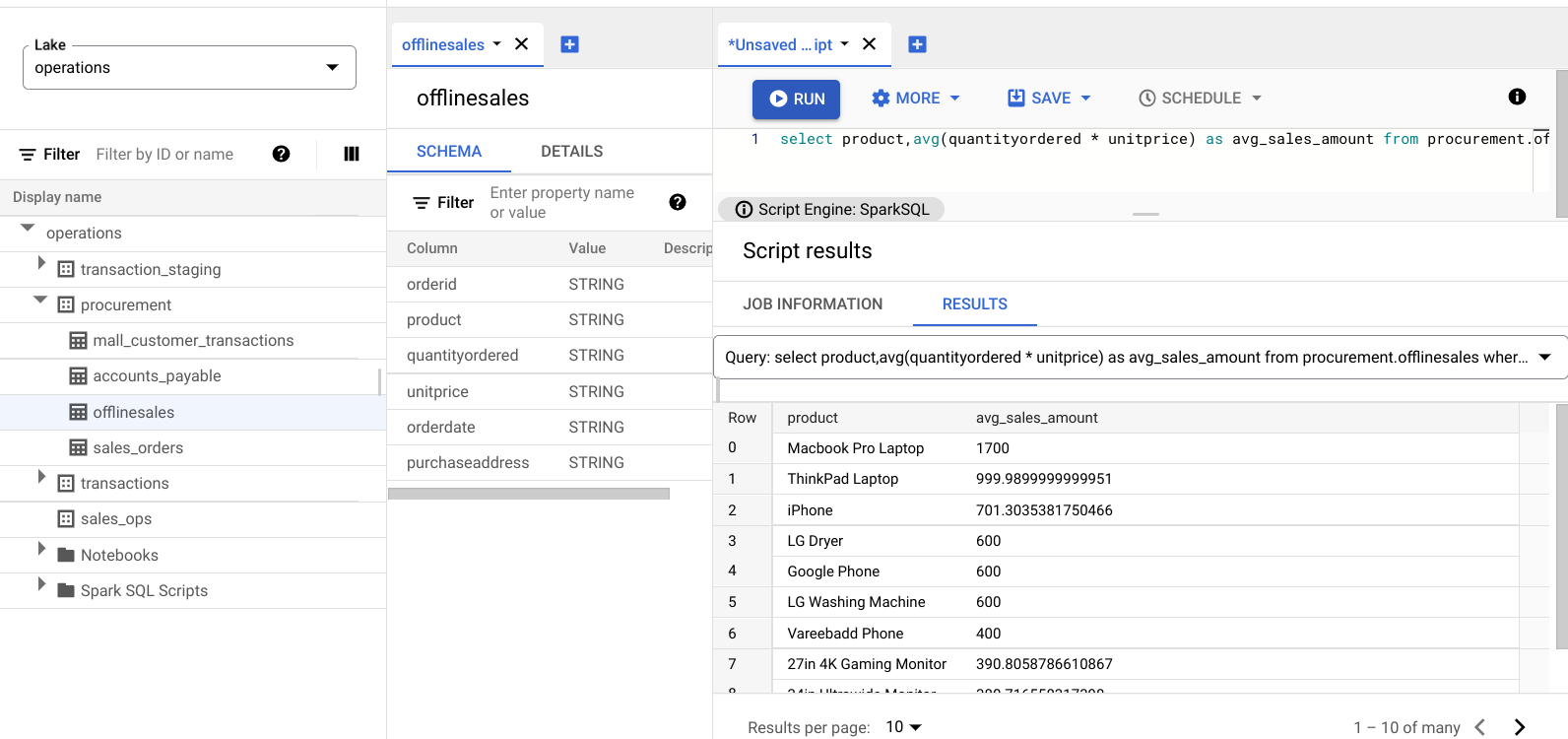
查找交易价值较高的产品

按产品类型和平均销售价格对销售情况进行细分，了解哪些产品的交易价值较高。

1. 输入以下查询：

   select product,avg(quantityordered * unitprice) as avg_sales_amount from procurement.offlinesales where orderid!='orderid' group by product order by avg_sales_amount desc;
   

2. 点击运行。

以下图片显示了 Results 窗格，该窗格使用名为 product 的列来识别交易价值较高的销售商品（显示在名为 avg_sales_amount 的列中）。

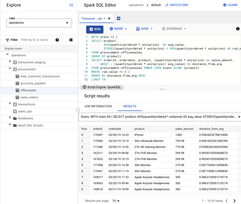
使用变异系数检测异常

上一个查询显示，笔记本电脑的平均交易金额较高。以下查询展示了如何检测数据集中非异常的笔记本电脑交易。

以下查询使用“方差系数”指标 rsd_value 来查找与平均值相比，值分布较低的非异常交易。标准差越小，异常值就越少。

1. 输入以下查询：

   WITH stats AS (
   SELECT product,
         AVG(quantityordered * unitprice)  AS avg_value,
         STDDEV(quantityordered * unitprice) / AVG(quantityordered * unitprice) AS rsd_value
   FROM procurement.offlinesales
   GROUP BY product)
   SELECT orderid, orderdate, product, (quantityordered * unitprice) as sales_amount,
       ABS(1 - (quantityordered * unitprice)/ avg_value) AS distance_from_avg
   FROM procurement.offlinesales INNER JOIN stats USING (product)
   WHERE rsd_value <= 0.2
   ORDER BY distance_from_avg DESC
   LIMIT 10
   

2. 点击运行。

3. 查看脚本结果。

   在下图中，“结果”窗格使用名为“商品”的列来识别交易价值在 0.2 的方差系数范围内的销售商品。

   

使用 JupyterLab 笔记本直观呈现异常

构建机器学习模型，以大规模检测和可视化异常。

1. 创建笔记本。

2. 在单独的标签页中打开该记事本，然后等待其加载。您执行 Spark SQL 查询的会话会继续。

3. 导入必要的软件包，并连接到包含交易数据的 BigQuery 外部表。运行以下代码：

   from google.cloud import bigquery
   from google.api_core.client_options import ClientOptions
   import os
   import warnings
   warnings.filterwarnings('ignore')
   import pandas as pd
   
   project = os.environ['GOOGLE_CLOUD_PROJECT']
   options = ClientOptions(quota_project_id=project)
   client = bigquery.Client(client_options=options)
   client = bigquery.Client()
   
   #Load data into DataFrame
   
   sql = '''select * from procurement.offlinesales limit 100;'''
   df = client.query(sql).to_dataframe()
   

4. 运行孤立森林算法，以发现数据集中的异常：

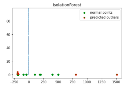
   to_model_columns = df.columns[2:4]
   from sklearn.ensemble import IsolationForest
   clf=IsolationForest(n_estimators=100, max_samples='auto', contamination=float(.12), \
                           max_features=1.0, bootstrap=False, n_jobs=-1, random_state=42, verbose=0)
   clf.fit(df[to_model_columns])
   pred = clf.predict(df[to_model_columns])
   df['anomaly']=pred
   outliers=df.loc[df['anomaly']==-1]
   outlier_index=list(outliers.index)
   #print(outlier_index)
   #Find the number of anomalies and normal points here points classified -1 are anomalous
   print(df['anomaly'].value_counts())
   

5. 使用 Matplotlib 可视化绘制预测的异常：

   import numpy as np
   from sklearn.decomposition import PCA
   pca = PCA(2)
   pca.fit(df[to_model_columns])
   res=pd.DataFrame(pca.transform(df[to_model_columns]))
   Z = np.array(res)
   plt.title("IsolationForest")
   plt.contourf( Z, cmap=plt.cm.Blues_r)
   b1 = plt.scatter(res[0], res[1], c='green',
                   s=20,label="normal points")
   b1 =plt.scatter(res.iloc[outlier_index,0],res.iloc[outlier_index,1], c='green',s=20,  edgecolor="red",label="predicted outliers")
   plt.legend(loc="upper right")
   plt.show()
   

此图片显示了交易数据，其中异常数据以红色突出显示。

安排笔记本

借助“探索”功能，您可以安排笔记本定期运行。按照相应步骤安排您创建的 Jupyter Notebook 的运行时间。

Dataplex 会创建一个调度任务来定期运行您的笔记本。如需监控任务进度，请点击查看时间表。

共享或导出笔记本

借助“探索”功能，您可以使用 IAM 权限与组织中的其他人共享记事本。

查看角色。向用户授予或撤消此笔记本的 Dataplex Viewer (roles/dataplex.viewer)、Dataplex Editor (roles/dataplex.editor) 和 Dataplex Administrator (roles/dataplex.admin) 角色。共享笔记本后，拥有数据湖级别查看者或编辑者角色的用户可以前往数据湖并处理共享的笔记本。

如需分享或导出笔记本，请参阅分享笔记本或导出笔记本。

清理

为避免因本教程中使用的资源导致您的 Google Cloud 账号产生费用，请删除包含这些资源的项目，或者保留项目但删除各个资源。

删除项目

注意：删除项目会产生以下影响：

• 项目中的所有内容都会被删除。如果您将现有项目用于本文档中的任务，则删除该项目后，还将删除您已在该项目中完成的任何其他工作。
• 自定义项目 ID 丢失。创建此项目时，您可能创建了要在将来使用的自定义项目 ID。要保留使用该项目 ID 的网址（例如 appspot.com 网址），请删除项目内的所选资源，而不是删除整个项目。

如果您打算探索多个架构、教程或快速入门，则重复使用项目可以帮助您避免超出项目配额限制。

Delete a Google Cloud project:

gcloud projects delete PROJECT_ID

逐个删除资源

1. 删除存储分区：

   gcloud storage buckets delete BUCKET_NAME

   重要提示：必须先清空存储桶，然后才能将其删除。
2. 删除实例：

   gcloud compute instances delete INSTANCE_NAME

后续步骤

• 详细了解 Dataplex Explore。
• 安排脚本和笔记本。