This page describes how to use evaluation metrics for your model after it is trained, and provides some basic suggestions for ways you might be able to improve model performance.
Introduction
After training a model, AutoML Tables uses the test dataset to evaluate the quality and accuracy of the new model, and provides an aggregate set of evaluation metrics indicating how well the model performed on the test dataset.
Using the evaluations metrics to determine the quality of your model depends on your business need and the problem you model is trained to solve. For example, there might be a higher cost to false positives than for false negatives, or vice versa. For regression models, does the delta between the prediction and the correct answer matter or not? These kinds of questions affect how you will look at your model evaluation metrics.
If you included a weight column in your training data, it does not affect evaluation metrics. Weights are considered only during the training phase.
Evaluation metrics for classification models
Classification models provide the following metrics:
AUC PR: The area under the precision-recall (PR) curve. This value ranges from zero to one, where a higher value indicates a higher-quality model.
AUC ROC: The area under the receiver operating characteristic (ROC) curve. This ranges from zero to one, where a higher value indicates a higher-quality model.
Accuracy: The fraction of classification predictions produced by the model that were correct.
Log loss: The cross-entropy between the model predictions and the target values. This ranges from zero to infinity, where a lower value indicates a higher-quality model.
F1 score: The harmonic mean of precision and recall. F1 is a useful metric if you're looking for a balance between precision and recall and there's an uneven class distribution.
Precision: The fraction of positive predictions produced by the model that were correct. (Positive predictions are the false positives and the true positives combined.)
Recall: The fraction of rows with this label that the model correctly predicted. Also called "True positive rate".
False positive rate: The fraction of rows predicted by the model to be the target label but aren't (false positive).
These metrics are returned for every distinct value of the target column. For multi-class classification models, these metrics are micro-averaged and returned as the summary metrics. For binary classification models, the metrics for the minority class are used as the summary metrics. The micro-averaged metrics are the expected value of each metric on a random sample from your dataset.
In addition to the above metrics, AutoML Tables provides two other ways to understand your classification model, the confusion matrix and a feature importance graph.
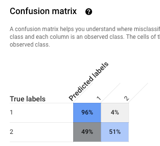
Confusion matrix: The confusion matrix helps you understand where misclassifications occur (which classes get "confused" with each other). Each row represents ground truth for a specific label, and each column shows the labels predicted by the model.
Confusion matrices are provided only for classification models with 10 or fewer values for the target column.
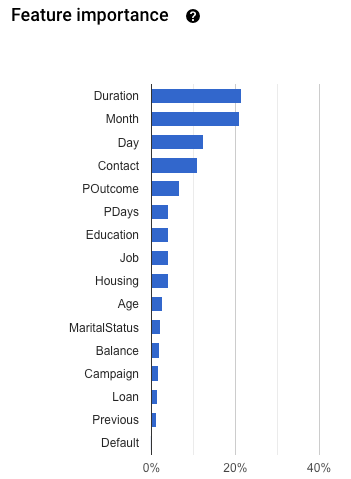
Feature importance: AutoML Tables tells you how much each feature impacts this model. It is shown in the Feature importance graph. The values are provided as a percentage for each feature: the higher the percentage, the more strongly that feature impacted model training.
You should review this information to ensure that all of the most important features make sense for your data and business problem. Learn more about explainability.
How micro-averaged precision is calculated
The micro-averaged precision is calculated by adding together the number of true positives (TP) for each potential value of the target column and dividing it by the number of true positives (TP) and true negatives (TN) for each potential value.
\[ precision_{micro} = \dfrac{TP_1 + \ldots + TP_n} {TP_1 + \ldots + TP_n + FP_1 + \ldots + FP_n} \]
where
- \(TP_1 + \ldots + TP_n\) is the sum of the true positives for each of n classes
- \(FP_1 + \ldots + FP_n\) is the sum of false positives for each of n classes
Score threshold
The score threshold is a number that ranges from 0 to 1. It provides a way to specify the minimum confidence level where a given prediction value should be taken as true. For example, if you have a class that is quite unlikely to be the actual value, then you would want to lower the threshold for that class; using a threshold of .5 or higher would result in that class being predicted extremely rarely (or never).
A higher threshold decreases false positives, at the expense of more false negatives. A lower threshold decreases false negatives at the expense of more false positives.
Put another way, the score threshold affects precision and recall. A higher threshold results in an increase in precision (because the model never makes a prediction unless it is extremely sure) but the recall (the percentage of positive examples that the model gets right) decreases.
Evaluation metrics for regression models
Regression models provide the following metrics:
MAE: The mean absolute error (MAE) is the average absolute difference between the target values and the predicted values. This metric ranges from zero to infinity; a lower value indicates a higher quality model.
RMSE: The root-mean-square error metric is a frequently used measure of the differences between the values predicted by a model or an estimator and the values observed. This metric ranges from zero to infinity; a lower value indicates a higher quality model.
RMSLE: The root-mean-squared logarithmic error metric is similar to RMSE, except that it uses the natural logarithm of the predicted and actual values plus 1. RMSLE penalizes under-prediction more heavily than over-prediction. It can also be a good metric when you don't want to penalize differences for large prediction values more heavily than for small prediction values. This metric ranges from zero to infinity; a lower value indicates a higher quality model. The RMSLE evaluation metric is returned only if all label and predicted values are non-negative.
r^2: r squared (r^2) is the square of the Pearson correlation coefficient between the labels and predicted values. This metric ranges between zero and one; a higher value indicates a higher quality model.
MAPE: Mean absolute percentage error (MAPE) is the average absolute percentage difference between the labels and the predicted values. This metric ranges between zero and infinity; a lower value indicates a higher quality model.
MAPE is not shown if the target column contains any 0 values. In this case, MAPE is undefined.
Feature importance: AutoML Tables tells you how much each feature impacts this model. It is shown in the Feature importance graph. The values are provided as a percentage for each feature: the higher the percentage, the more strongly that feature impacted model training.
You should review this information to ensure that all of the most important features make sense for your data and business problem. Learn more about explainability.
Getting the evaluation metrics for your model
To evaluate how well your model did on the test dataset, you inspect the evaluation metrics for your model.
Console
To see your model's evaluation metrics using the Google Cloud console:
Go to the AutoML Tables page in the Google Cloud console.
Select the Models tab in the left navigation pane, and select the model you want to get the evaluation metrics for.
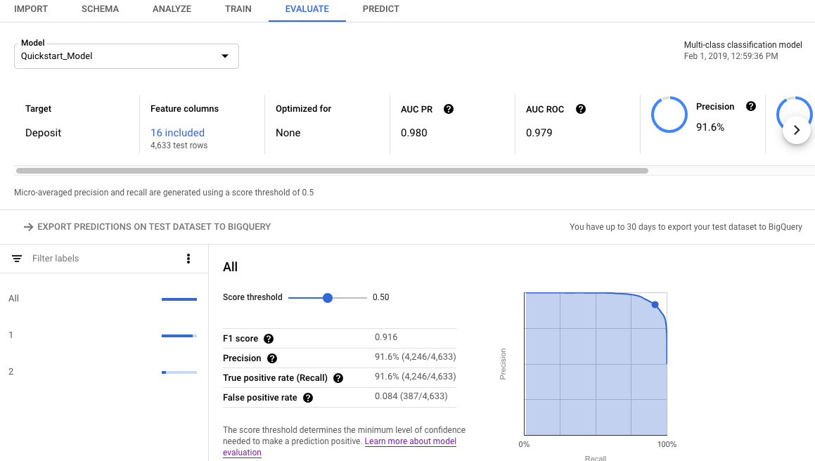
Open the Evaluate tab.
The summary evaluation metrics are displayed across the top of the screen. For binary classification models, the summary metrics are the metrics of the minority class. For multi-class classification models, the summary metrics are the micro-averaged metrics.
For classification metrics, you can click on individual target values to see the metrics for that value.
REST
To get evaluation metrics for your model using the Cloud AutoML API, you use the modelEvaluations.list method.
Before using any of the request data, make the following replacements:
-
endpoint:
automl.googleapis.comfor the global location, andeu-automl.googleapis.comfor the EU region. - project-id: your Google Cloud project ID.
- location: the location for the resource:
us-central1for Global oreufor the European Union. -
model-id: the ID of the model you want to evaluate. For example,
TBL543.
HTTP method and URL:
GET https://endpoint/v1beta1/projects/project-id/locations/location/models/model-id/modelEvaluations/
To send your request, choose one of these options:
curl
Execute the following command:
curl -X GET \
     -H "Authorization: Bearer $(gcloud auth print-access-token)" \
     -H "x-goog-user-project: project-id" \
     "https://endpoint/v1beta1/projects/project-id/locations/location/models/model-id/modelEvaluations/"
PowerShell
Execute the following command:
$cred = gcloud auth print-access-token
$headers = @{ "Authorization" = "Bearer $cred"; "x-goog-user-project" = "project-id" }

Invoke-WebRequest `
    -Method GET `
    -Headers $headers `
    -Uri "https://endpoint/v1beta1/projects/project-id/locations/location/models/model-id/modelEvaluations/" | Select-Object -Expand Content
Java
If your resources are located in the EU region, you must explicitly set the endpoint. Learn more.
Node.js
If your resources are located in the EU region, you must explicitly set the endpoint. Learn more.
Python
The client library for AutoML Tables includes additional Python methods that simplify using the AutoML Tables API. These methods refer to datasets and models by name instead of id. Your dataset and model names must be unique. For more information, see the Client reference.
If your resources are located in the EU region, you must explicitly set the endpoint. Learn more.
Understanding evaluation results using the API
When you use the Cloud AutoML API to get model evaluation metrics, a large amount of information is returned. Understanding how the metrics results are structured can help you interpret the results and use them to evaluate your model.
Classification results
For a classification model, the results include multiple ModelEvaluation objects, each of which contains multiple ConfidenceMetricsEntry objects. Understanding how the results are structured helps you choose the correct objects to use when evaluating your model.
Two ModelEvaluation objects are returned for each distinct value of the target column present in the training data. In addition, there are two summary ModelEvaluation objects, and one empty ModelEvaluation object that can be ignored.
The two ModelEvaluation objects returned for a specific label value show the
label value in the displayName field. They each use different
position threshold values: one, and MAX_INT (the highest possible number). The
position threshold determines how many outcomes are considered for a prediction.
For a classification problem, using a position threshold of one often makes the
most sense, because there is only one label chosen for each input. For
multi-label problems, more than one label can be chosen per input, so the
evaluation metrics returned for the MAX_INT position threshold might be more
useful. You should determine which metrics to use based on the specific use case
of your model.
The two summary ModelEvaluation objects do not include the displayName field,
except as part of the confusion matrix. Also, their value for the
evaluatedExampleCount field is the total number of rows in the training data.
For multi-class classification models the summary objects provide the
micro-averaged metrics based on all of the per-label metrics.
For binary classification models, the metrics for the minority class are used as
the summary metrics. Use the ModelEvaluation object with a position threshold of
one for your summary metrics.
Each ModelEvaluation object contains up to 100 ConfidenceMetricsEntry objects, depending on the training data. Each ConfidenceMetricsEntry object provides a different value for the confidence threshold (also called the score threshold).
Summary ModelEvaluation objects look similar to the following example. Note that the field display order can differ.
model_evaluation {
  name: "projects/8628/locations/us-central1/models/TBL328/modelEvaluations/18011"
  create_time {
    seconds: 1575513478
    nanos: 163446000
  }
  evaluated_example_count: 1013

  classification_evaluation_metrics {

    au_roc: 0.99749845
    log_loss: 0.01784837
    au_prc: 0.99498594

    confidence_metrics_entry {
      recall: 0.99506414
      precision: 0.99506414
      f1_score: 0.99506414
      false_positive_rate: 0.002467917
      true_positive_count: 1008
      false_positive_count: 5
      false_negative_count: 5
      true_negative_count: 2021
      position_threshold: 1
    }
    confidence_metrics_entry {
      confidence_threshold: 0.0149591835
      recall: 0.99506414
      precision: 0.99506414
      f1_score: 0.99506414
      false_positive_rate: 0.002467917
      true_positive_count: 1008
      false_positive_count: 5
      false_negative_count: 5
      true_negative_count: 2021
      position_threshold: 1
    }
   ...
   confusion_matrix {
      row {
        example_count: 519
        example_count: 2
        example_count: 0
      }
      row {
        example_count: 3
        example_count: 75
        example_count: 0
      }
      row {
        example_count: 0
        example_count: 0
        example_count: 414
      }
      display_name: "RED"
      display_name: "BLUE"
      display_name: "GREEN"
    }
  }
}
Label-specific ModelEvaluation objects look similar to the following example. Note that the field display order can differ.
model_evaluation {
  name: "projects/8628/locations/us-central1/models/TBL328/modelEvaluations/21860"
  annotation_spec_id: "not available"
  create_time {
    seconds: 1575513478
    nanos: 163446000
  }
  evaluated_example_count: 521

  classification_evaluation_metrics {

    au_prc: 0.99933827
    au_roc: 0.99889404
    log_loss: 0.014250426

    confidence_metrics_entry {
      recall: 1.0
      precision: 0.51431394
      f1_score: 0.6792699
      false_positive_rate: 1.0
      true_positive_count: 521
      false_positive_count: 492
      position_threshold: 2147483647
    }
    confidence_metrics_entry {
      confidence_threshold: 0.10562216
      recall: 0.9980806
      precision: 0.9904762
      f1_score: 0.9942639
      false_positive_rate: 0.010162601
      true_positive_count: 520
      false_positive_count: 5
      false_negative_count: 1
      true_negative_count: 487
      position_threshold: 2147483647
    }
  ...
  }
  display_name: "RED"
}
Regression results
For a regression model, you should see output similar to the following example:
{
  "modelEvaluation": [
    {
      "name": "projects/1234/locations/us-central1/models/TBL2345/modelEvaluations/68066093",
      "createTime": "2019-05-15T22:33:06.471561Z",
      "evaluatedExampleCount": 418
    },
    {
      "name": "projects/1234/locations/us-central1/models/TBL2345/modelEvaluations/852167724",
      "createTime": "2019-05-15T22:33:06.471561Z",
      "evaluatedExampleCount": 418,
      "regressionEvaluationMetrics": {
        "rootMeanSquaredError": 1.9845301,
        "meanAbsoluteError": 1.48482,
        "meanAbsolutePercentageError": 15.155516,
        "rSquared": 0.6057632,
        "rootMeanSquaredLogError": 0.16848126
      }
    }
  ]
}
Troubleshooting model issues
Model evaluation metrics should be good, but not perfect. Poor model performance and perfect model performance are both indications that something went wrong with the training process.
Poor performance
If your model is not performing as well as you would like, here are some things to try.
Review your schema.
Make sure all your columns have the correct type, and that you excluded from training any columns that were not predictive, such as ID columns.
Review your data
Missing values in non-nullable columns cause that row to be ignored. Make sure your data does not have too many errors.
Export the test dataset and examine it.
By inspecting the data and analyzing when the model is making incorrect predictions, you might determine that you need more training data for a particular outcome, or that your training data introduced leakage.
Increase the amount of training data.
If you don't have enough training data, model quality suffers. Make sure your training data is as unbiased as possible.
Increase the training time
If you had a short training time, you might get a higher-quality model by allowing it to train for a longer period of time.
Perfect performance
If your model returned near-perfect evaluation metrics, something might be wrong with your training data. Here are some things to look for:
Target leakage
Target leakage happens when a feature is included in the training data that cannot be known at training time, and which is based on the outcome. For example, if you included a Frequent Buyer number for a model trained to decide whether a first-time user would make a purchase, that model would have very high evaluation metrics, but would perform poorly on real data, because the Frequent Buyer number could not be included.
To check for target leakage, review the Feature importance graph on the Evaluate tab for your model. Make sure the columns with high importance are truly predictive and are not leaking information about the target.
Time column
If the time of your data matters, make sure you used a Time column or a manual split based on time. Not doing so can skew your evaluation metrics. Learn more.
Downloading your test dataset to BigQuery
You can download your test dataset, including the target column, along with the model's result for each row. Inspecting the rows that the model got wrong can provide clues for how to improve the model.
Open AutoML Tables in the Google Cloud console.
Select Models in the left navigation pane and click your model.
Open the Evaluate tab and click Export predictions on test dataset to BigQuery.
After the export completes, click View your evaluation results in BigQuery to see your data.
What's next
- Deploy your model to get online predictions.
- Get batch predictions from your model.