BigQuery explained: How to query your data
Rajesh Thallam
Solutions Architect, Generative AI Solutions
Previously in BigQuery Explained, we reviewed BigQuery architecture, storage management, and ingesting data into BigQuery. In this post, we will cover querying datasets in BigQuery using SQL, saving and sharing queries, creating views and materialized views. Let’s get started!
Standard SQL
BigQuery supports two SQL dialects: standard SQL and legacy SQL. Standard SQL is preferred for querying data stored in BigQuery because it’s compliant with the ANSI SQL 2011 standard. It has other advantages over legacy SQL, such as automatic predicate push down for JOIN operations and support for correlated subqueries. Refer to Standard SQL highlights for more information.
When you run a SQL query in BigQuery, it automatically creates, schedules and runs a query job. BigQuery runs query jobs in two modes: interactive (default) and batch.
Interactive (on-demand) queries are executed as soon as possible, and these queries count towards concurrent rate limit and daily limit.
Batch queries are queued and started as soon as idle resources are available in the BigQuery shared resource pool, which usually occurs within a few minutes. If BigQuery hasn’t started the query within 24 hours, job priority is changed to interactive. Batch queries don’t count towards your concurrent rate limit. They use the same resources as interactive queries.
The queries in this post follow Standard SQL dialect and run in interactive mode, unless otherwise mentioned.

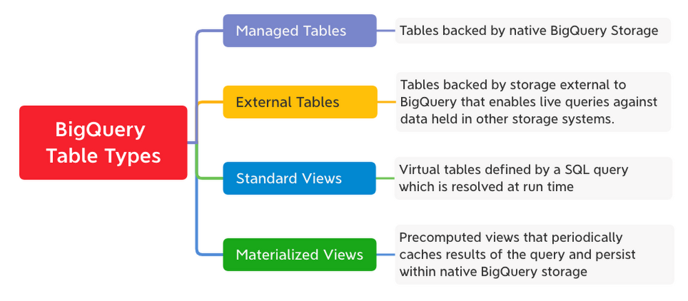
BigQuery Table Types
Every table in BigQuery is defined by a schema describing the column names, data types, and other metadata. BigQuery supports the following table types:
BigQuery Schemas
In BigQuery, schemas are defined at the table level and provide structure to the data. Schema describes column definitions with their name, data type, description and mode.
- Data types can be simple data types, such as integers, or more complex, such as
ARRAYandSTRUCTfor nested and repeated values. - Column modes can be
NULLABLE,REQUIRED, orREPEATED.
Table schema is specified when loading data into the table or when creating an empty table. Alternatively, when loading data, you can use schema auto-detection for self-describing source data formats such as Avro, Parquet, ORC, Cloud Firestore or Cloud Datastore export files. Schema can be defined manually or in a JSON file as shown.
Using SQL for Analysis
Now let’s analyze one of the public BigQuery datasets related to NCAA Basketball games and players using SQL. The game data covers play-by-play and box scores dated back to 2009. We will look at a specific game from the 2014 season between Kentucky’s Wildcats and Notre Dame’s Fighting Irish. This game had an exciting finish. Let’s find out what made it exciting!
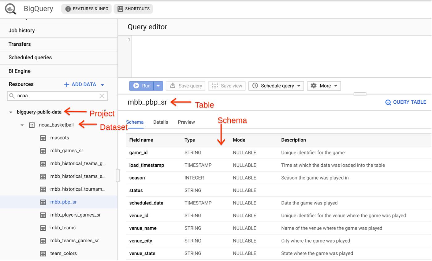
On your BigQuery Sandbox, open the NCAA Basketball dataset from public datasets. Click on the “VIEW DATASET” button to open the dataset in BigQuery web UI.Navigate to table mbb_pbp_sr under ncaa_basketball dataset to look at the schema. This table has play-by-play information of all men’s basketball games in the 2013–2014 season, and each row in the table represents a single event in a game.
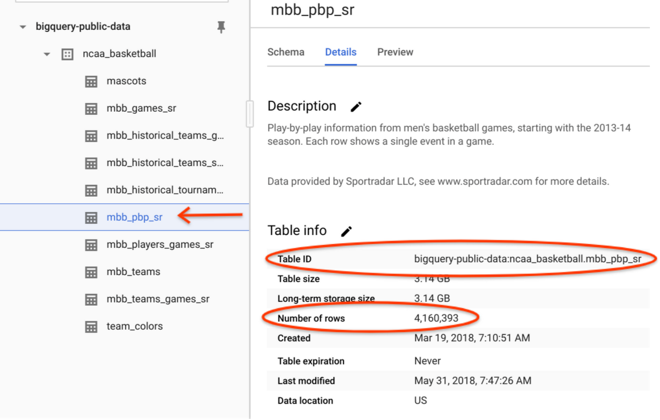
Check the Details section of table mbb_pbp_sr. There are ~4 million game events with a total volume of ~3GB.
Let’s run a query to filter the events for the game we are interested in. The query selects the following columns from the mbb_pbp_sr table:
game_clock: Time left in the game before the finishpoints_scored: Points were scored in an eventteam_name: Name of the team who scored the pointsevent_description: Description about the eventtimestamp: Time when the event occurred
A breakdown of what this query is doing:
The
SELECTstatement retrieves the rows and the specified columnsFROMthe tableThe
WHEREclause filters the rows returned bySELECT. This query filters to return rows for the specific game we are interested in.The
ORDER BYstatement controls the order of rows in the result set. This query sorts the rows resulting fromSELECTby timestamp in descending order.Finally, the
LIMITconstraints the amount of data returned from the query. This query returns 10 events from the results set after the rows are sorted. Note that addingLIMITdoes not reduce the amount of data processed by the query engine.
Now let’s look at the results.
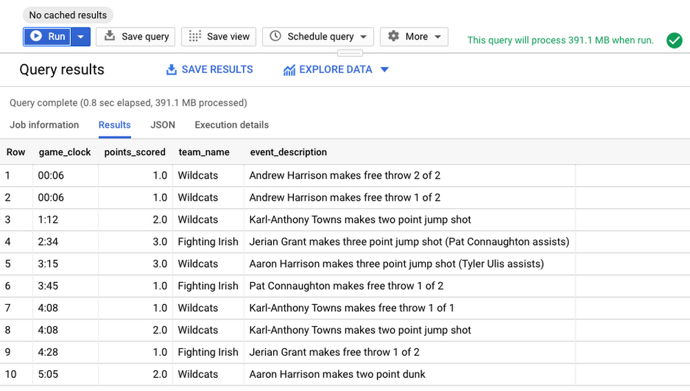
From the results, it appears the player Andrew Harrison made two free throws scoring 2 points with only 6 seconds remaining in the game. This doesn’t tell us much except there were points scored towards the very end of the game.
Tip: Avoid using SELECT * in the query. Instead query only the columns needed. To exclude only certain columns use SELECT * EXCEPT.
Let’s modify the query to include cumulative sum of scores for each team rolling up to the event time, using analytic (window) functions. Analytic functions computes aggregates for each row over a group of rows defined by a window whereas aggregate functions compute a single aggregate value over a group of rows.
Run the below query with two new columns added—wildcats_score and fighting_irish_score, calculated on-the-fly using points_scored column.
A breakdown of what this query is doing:
Calculate cumulative
SUMof scores by each team in the game—specified byCASEstatementSUMis calculated on scores in the window defined withinOVERclauseOVERclause references a window (group of rows) to useSUMORDER BYis part of window specification that defines sort order within a partition. This query orders rows bytimestampDefine the window frame from the start of the game specified by
UNBOUNDED PRECEDINGto theCURRENT ROWover which the analytic functionSUM()is evaluated.
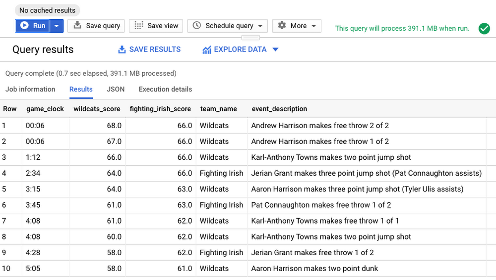
From the results, we can see how the game ended. The Fighting Irish held the lead by four points with 04:28 minutes remaining. Karl-Anthony Towns of Wildcats was able to tie the game on a layup with 01:12 minutes remaining, and Andrew Harrison made two free throws with 00:06 seconds remaining, setting the stage for the Wildcats’ win. That was a nail biting finish indeed!
In addition to aggregate and analytic functions, BigQuery also supports functions and operators such as string manipulation, date/time, mathematical functions, JSON extract and more, as shown.
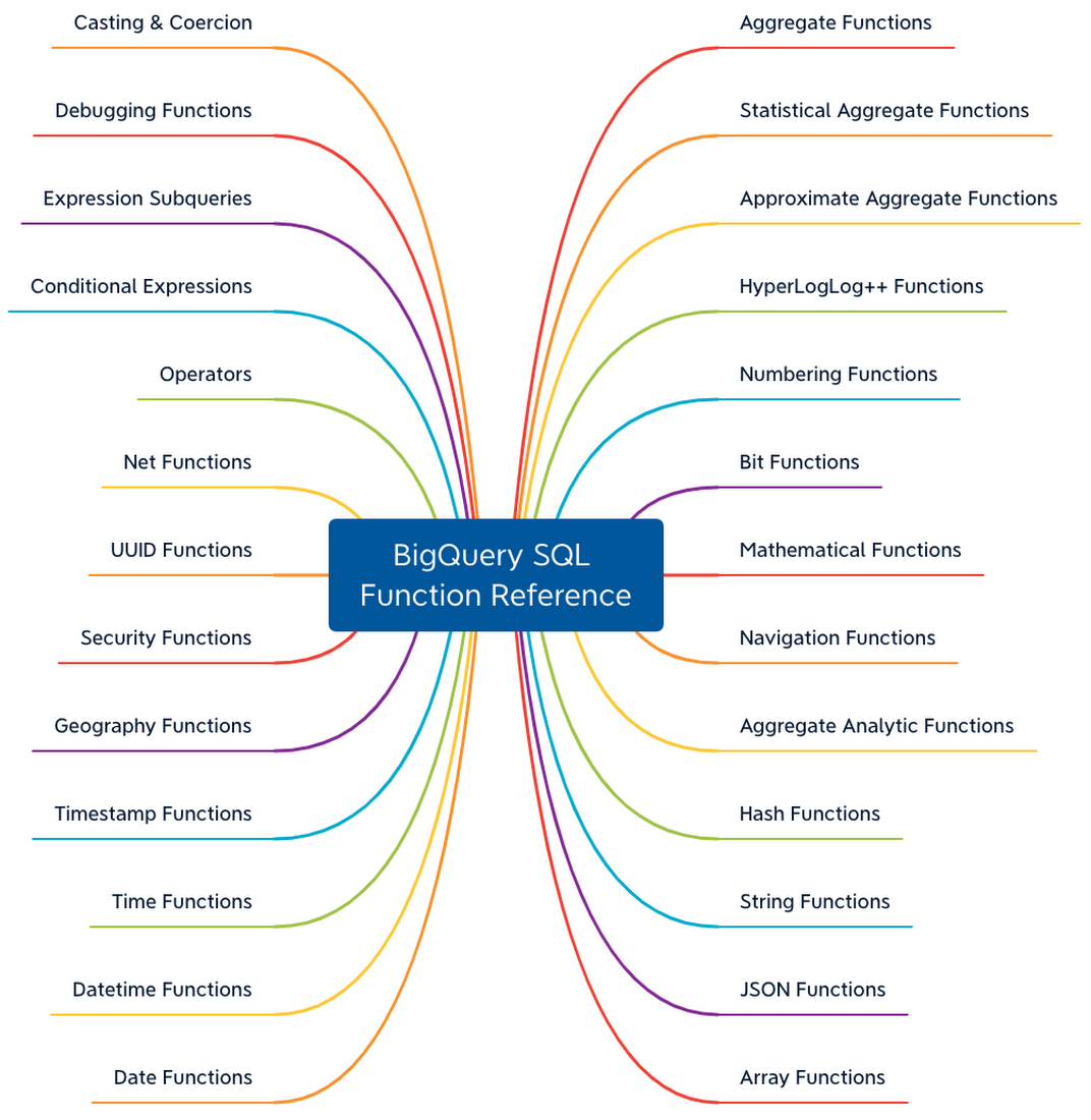
Refer BigQuery SQL function reference for the complete list. In the upcoming posts, we will cover other advanced query features in BigQuery such as User Defined Functions, Spatial functions and more.
The Life of a BigQuery SQL Query
Under the hood when you run the SQL query it does the following:
A QueryJob is submitted to the BigQuery service. As reviewed in the BigQuery architecture, the BigQuery compute is decoupled from the BigQuery storage, and they are designed to work together to organize the data to make queries efficient over huge datasets.
Each query executed is broken up into stages which are then processed by workers (slots) and written back out to Shuffle. Shuffle provides resilience to failures within workers themselves, say a worker were to have an issue during query processing.
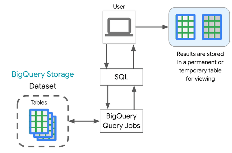
BigQuery engine utilizes BigQuery’s columnar storage format to scan only the required columns to run the query. One of the best practices to control costs is to query only the columns that you need.
After the query execution is completed, the query service persists the results into a temporary table, and the web UI displays that data. You can also request to write results into a permanent table.
Saving and Sharing Queries
Saving Queries
Now that you have run SQL queries to perform analysis, how would you save those results? BigQuery writes all query results to a table. The table is either explicitly identified by the user as a destination table or a temporary cached results table. This temporary table is stored for 24 hours, so if you run the exact same query again (exact string match), and if the results would not be different, then BigQuery will simply return a pointer to the cached results. Queries that can be served from the cache do not incur any charges. Refer to the documentation to understand limitations and exceptions to query caching.
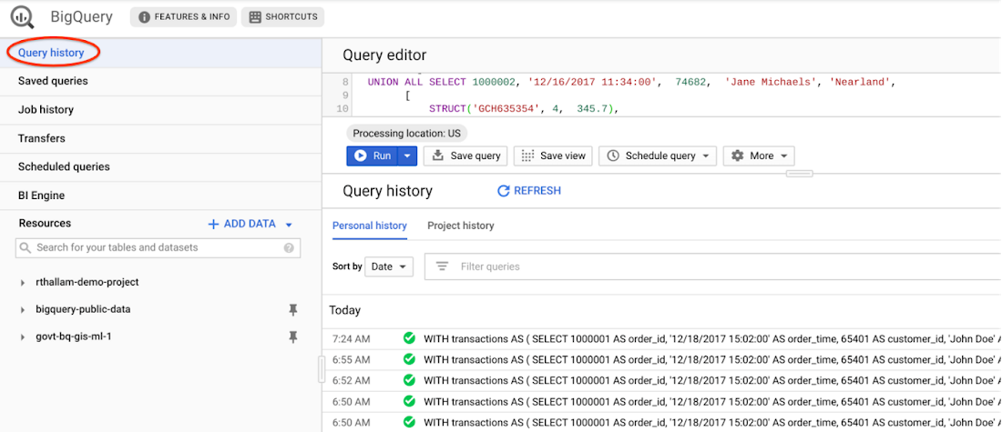
You can view cached query results from the Query History tab on BigQuery UI. This history includes all queries submitted by you to the service, not just those submitted via the web UI.
You can disable retrieval of cached results from the query settings when executing the query. This requires BigQuery to compute the query result, which will result in charges for the query to execute. This is typically used in benchmarking scenarios, such as in the previous post comparing performance of partitioned and clustered tables against non-partitioned tables.
You can also request the query write to a destination table. You will have control on when the table is deleted. Because the destination table is permanent, you will be charged for the storage of the results.
Sharing Queries
BigQuery allows you to share queries with others. When you save a query, it can be private (visible only to you), shared at the project level (visible to project members), or public (anyone can view it).
Check this video to know how to save and share your queries in BigQuery.

Standard Views
A view is a virtual table defined by a SQL query. A view has properties similar to a table and can be queried as a table. The schema of the view is the schema that results from running the query. The query results from the view contain data only from the tables and fields specified in the query that defines the view.
You can create a view by saving the query from the BigQuery UI using the “Save View” button or using BigQuery DDL—CREATE VIEW statement. Saving a query as a view does not persist results aside from the caching to a temporary table, which expires within a 24 hour window. The behavior is similar to the query executed on the tables.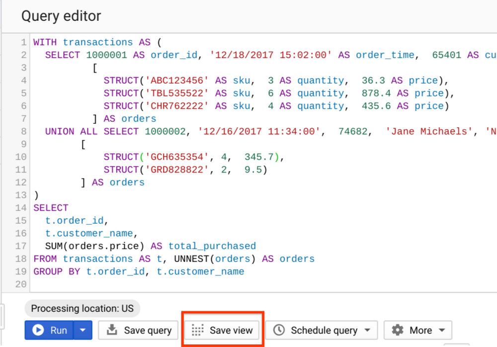
When to use standard Views?
- Let’s say you want to expose queries with complex logic to your users and you want to avoid the users needing to remember the logic, then you can roll those queries into a view.
- Another use case is—views can be placed into datasets and offer fine-grained access controls to share dataset with specific users and groups without giving them access to underlying tables. These views are called authorized views. We will look into securing and accessing datasets in detail in a future post.
Materialized Views
BigQuery supports Materialized Views (MV)—a beta feature. MV are precomputed views that periodically cache results of a query for increased performance and efficiency. Queries using MV are generally faster and consume less resources than queries retrieving the same data only from the base table. They can significantly boost performance of workloads with common and repeated queries.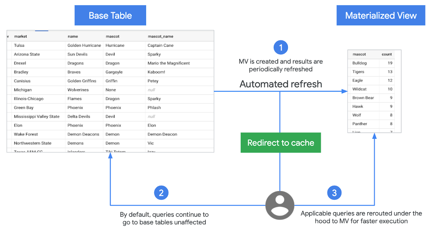
Following are the key features of materialized views:
Zero Maintenance
BigQuery leverages precomputed results from MV and whenever possible reads only delta changes from the base table to compute up-to-date results. It automatically synchronizes data refreshes with data changes in base tables. No user inputs required. You also have the option to trigger manual refresh the views to control the costs of refresh jobs.
Always fresh
MV is always consistent with the source table. They can be queried directly or can be used by the BigQuery optimizer to process queries to the base tables.
Smart Tuning
MV supports query rewrites. If a query against the source table can instead be resolved by querying the MV, BigQuery will rewrite (reroute) the query to the MV for better performance and/or efficiency.
You create MV using BigQuery DDL—CREATE MATERIALIZED VIEW statement.
When to use Materialized Views?
MV are suited for cases when you need to query the latest data while cutting down latency and cost by reusing the previously computed results. MV act as pseudo-indexes, accelerating queries to the base table without updating any existing workflows.
Limitations of Materialized Views
As of this writing, joins are not currently supported in MV. However, you can leverage MV in a query that does aggregation on top of joins. This reduces cost and latency of the query.
MV supports a limited set of aggregation functions and restricted SQL. Refer the query patterns supported by materialized views.
Refer to BigQuery documentation for working with materialized views, and best practices.
What Next?
In this post, we reviewed the lifecycle of a SQL query in BigQuery, working with window functions, creating standard and materialized views, saving and sharing queries.
References
BigQuery Functions reference
Analytic (window) functions in BigQuery
Standard views in BigQuery [Docs]
Materialized views in BigQuery [Docs]
BigQuery best practices for query performance
Codelab
Try this codelab to query a large public dataset based on Github archives.
In the next post, we will dive into joins, optimizing join patterns and denormalizing data with nested and repeated data structures.
Stay tuned. Thank you for reading! Have a question or want to chat? Find me on Twitter or LinkedIn.
Thanks to Yuri Grinshsteyn and Alicia Williams for helping with the post.
The complete BigQuery Explained series
- BigQuery explained: An overview of BigQuery's architecture
- BigQuery explained: Storage overview, and how to partition and cluster your data for optimal performance
- BigQuery explained: How to ingest data into BigQuery so you can analyze it
- BigQuery explained: How to query your data
- BigQuery explained: Working with joins, nested & repeated data
- BigQuery explained: How to run data manipulation statements to add, modify and delete data stored in BigQuery