BigQuery explained: Storage overview, and how to partition and cluster your data for optimal performance

In the previous post of BigQuery Explained series, we reviewed the high level architecture of BigQuery and showed how to get started with BigQuery. In this post, we will look at the BigQuery storage organization, storage format and introduce one of the best practices of BigQuery to partition and cluster your data for optimal performance. Let’s dive right into it!

BigQuery Resource Model

BigQuery organizes data tables into units called datasets. These datasets are scoped to your GCP project. These multiple scopes—project, dataset, and table—helps you structure your information logically. You can use multiple datasets to separate tables pertaining to different analytical domains, and you can use project-level scoping to isolate datasets from each other according to your business needs.

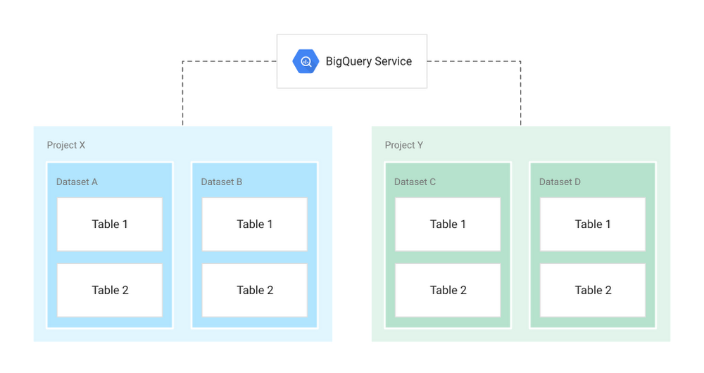
Projects

• Root namespace for objects

• Contain multiple datasets, jobs, access control lists and IAM roles

• Control billing, users, and user privileges

Datasets

• Collections of “related” tables/views together with labels and description

• Allow storage access control at Dataset level

• Define location of data i.e. multi-regional (US, EU) or regional (asia-northeast1)

Tables

• Collections of columns and rows stored in managed storage

• Defined by a schema with strongly-typed columns of values

• Allow access control at Table level and Column level

Views

• Virtual tables defined by a SQL query

• Allow access control at View level

Jobs

• Actions run by BigQuery on your behalf—load data, export data, copy data, or query data

• Jobs are executed asynchronously

When you reference a table from the command line, in SQL queries, or in code, you refer to it by using the following construct: project.dataset.table.

Storage Management

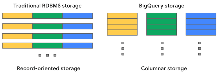
BigQuery uses variations and advancements on columnar storage. Internally, BigQuery stores data in a proprietary columnar format called Capacitor, which has a number of benefits for data warehouse workloads. BigQuery uses a proprietary format because the storage engine can evolve in tandem with the query engine, which takes advantage of deep knowledge of the data layout to optimize query execution. Each column in the table is stored in a separate file block and all the columns are stored in a single capacitor file, which are compressed and encrypted on disk. BigQuery uses query access patterns to determine the optimal number of physical shards and how data is encoded.

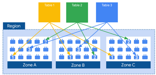
The actual persistence layer is provided by Google’s distributed file system, Colossus, where data is automatically compressed, encrypted, replicated, and distributed. Colossus ensures durability using erasure encoding to store redundant chunks of data on multiple physical disks. This is all accomplished without impacting the computing power available for your queries. Separating storage from compute allows you to scale to petabytes in storage seamlessly, without requiring additional expensive compute resources. There are a number of other benefits of decoupling compute and storage.

Take Advantage of Long-Term Storage

You can load data into BigQuery at no cost (for batch loads) because BigQuery storage costs are based on the amount of data stored (first 10 GB is free each month) and whether storage is considered active or long-term.

• If you have a table or partition modified in the last 90 days, it is considered as active storage and incurs a monthly charge for data stored at BigQuery storage rates.

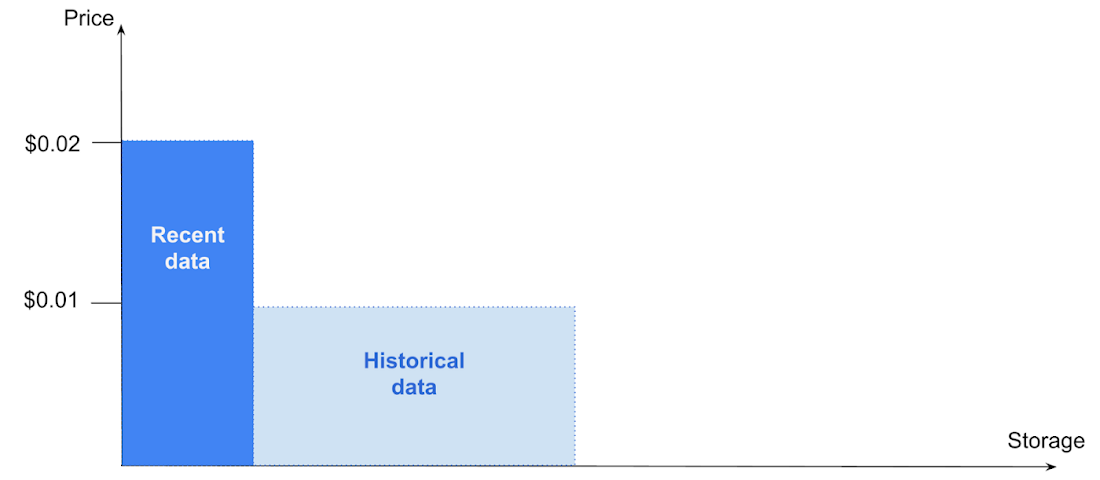
A best practice when optimizing costs is to keep your data in BigQuery. Rather than exporting your older data to another storage option (such as Cloud Storage), take advantage of BigQuery’s long-term storage pricing. This means not having to delete old data or architect a data archival process. Since the data remains in BigQuery, you can also query older data using the same interface, at the same cost levels, with the same performance characteristics.

Partitioning and Clustering

Keeping data in BigQuery is a best practice if you’re looking to optimize both cost and performance. Another best practice is using BigQuery’s table partitioning and clustering features to structure your data to match common data access patterns.

Partitioning

A partitioned table is a special table that is divided into segments, called partitions, that make it easier to manage and query your data. You can typically split large tables into many smaller partitions using data ingestion time or TIMESTAMP/DATE column or an INTEGER column. BigQuery’s decoupled storage and compute architecture leverages column-based partitioning simply to minimize the amount of data that slot workers read from disk. Once slot workers read their data from disk, BigQuery can automatically determine more optimal data sharding and quickly repartition data using BigQuery’s in-memory shuffle service.

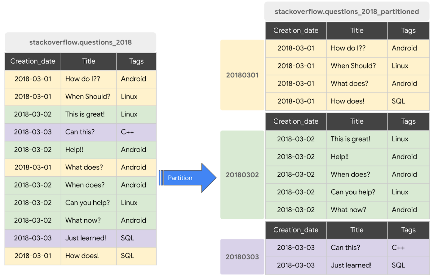
Data written to a column-based time partitioned table is automatically delivered to the appropriate partition based on the value of the data. Similarly, queries that express filters on the partitioning column can reduce the overall data scanned, which can yield improved performance and reduced query cost for on-demand queries.

BigQuery supports following ways to create partitioned tables

Ingestion time partitioned tables

• Partitioned on the data’s ingestion time or arrival time.

• BigQuery automatically loads data into daily, date based partitions reflecting the data’s ingestion or arrival time.

• BigQuery adds two pseudo columns to ingestion-time partitioned tables—a _PARTITIONTIME pseudo column containing a date-based timestamp for data and a _PARTITIONDATE pseudo column contains a date representation.
  

DATE/TIMESTAMP column partitioned tables

• Partitioned based on a TIMESTAMP or DATE column.
  

• BigQuery routes data to the appropriate partition based on the date value (expressed in UTC) in the partitioning column.

• BigQuery creates two special partitions: the __NULL__ partition for capturing rows NULL values in the partitioning column and the __UNPARTITIONED__ partition for data outside the allowed range of dates.

• You can create partitions with granularity starting from hourly partitioning.

INTEGER range partitioned tables

• Partitioned based on an integer column with start, end, and interval values.

• BigQuery creates two special partitions: the __NULL__ partition for capturing rows NULL values in the partitioning column and the __UNPARTITIONED__ partition for data outside the allowed range of integers.

Let’s look at partitioning in action. To see the difference in performance between a non-partitioned and a partitioned table, we will create non-partitioned and partitioned tables with the same dataset and check the query performance.

Before Partitioning

By running the following SQL query, we will create a non-partitioned table with data loaded from a public data set based on StackOverflow posts by creating a new table from an existing table. This table will contain the StackOverflow posts created in 2018.

Let’s query the non-partitioned table to fetch all StackOverflow questions tagged with ‘android’ in the month of January 2018.

Before the query runs, caching is disabled to be fair when comparing performance with partitioned and clustered tables.

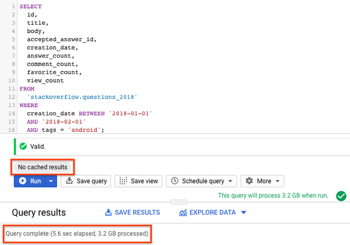
From the query results, you can see that the query on a non-partitioned table took 5.6s to scan the entire 3.2GB of data with StackOverflow posts created in 2018.

Partition the Table

Now let’s see whether partitioned tables can do better. You can create partitioned tables in multiple ways. We will create a DATE/TIMESTAMP partitioned table using BigQuery DDL statements. We chose the partitioning column as creation_date based on the query access pattern.

Now let’s run the previous query on the partitioned table, with cache disabled, to fetch all StackOverflow questions tagged with ‘android’ in the month of January 2018.

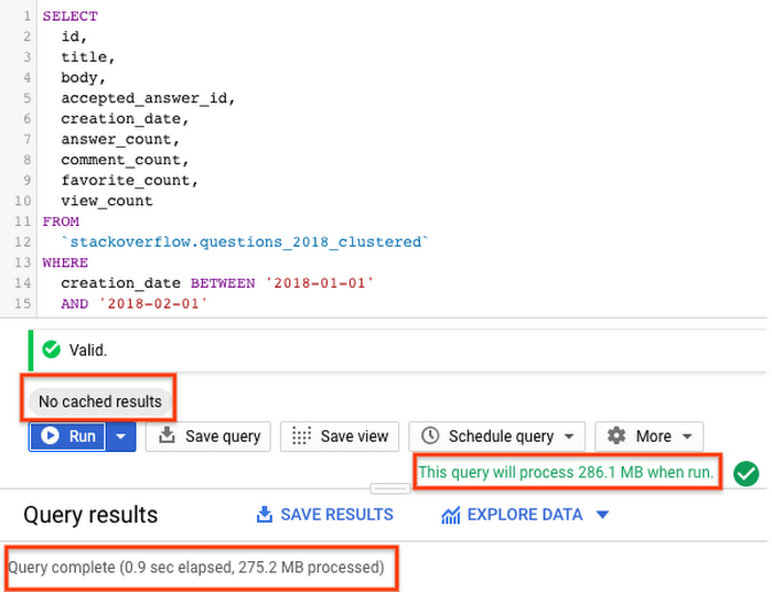
With partitioned table query scanned only the required partitions in <2s processing ~290MB data compared to query running with non-partitioned table processing 3.2GB.

Partition management is key to fully maximizing BigQuery performance and cost when querying over a specific range—it results in scanning less data per query, and pruning is determined before query start time. While partitioning reduces cost and improves performance, it also prevents cost explosion due to user accidentally querying really large tables in entirety.

Tip: You can control and optimize storage costs by configuring table expiration to remove unneeded tables and partitions.

Learn more about partitioned tables here.

Clustering

When a table is clustered in BigQuery, the table data is automatically organized based on the contents of one or more columns in the table’s schema. The columns you specify are used to collocate related data. Usually high cardinality and non-temporal columns are preferred for clustering.

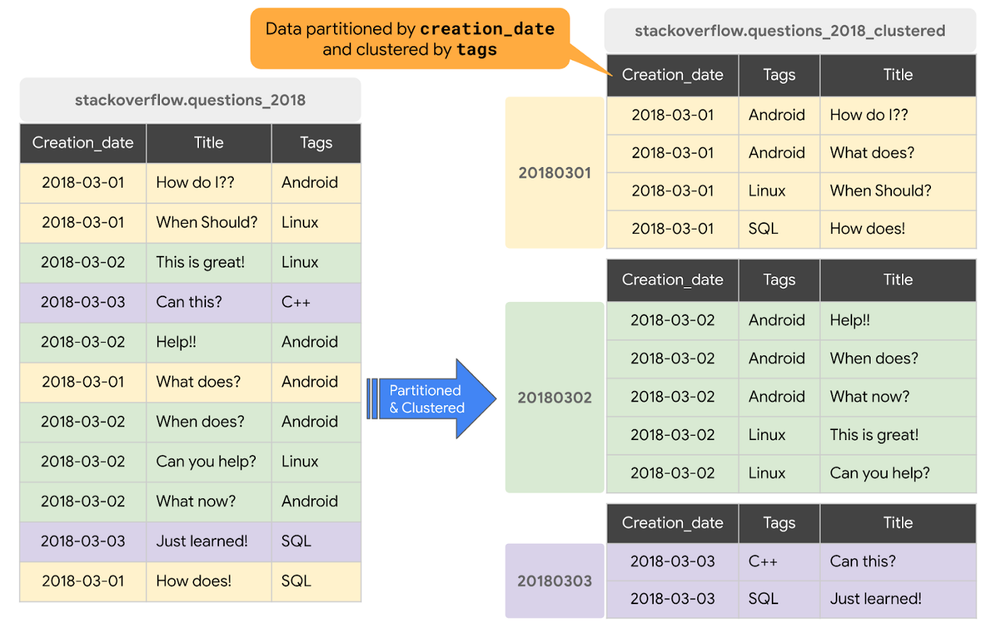
Clustering can improve the performance of certain types of queries, such as those using filter clauses and queries aggregating data.

• When a query containing a filter clause filters data based on the clustering columns, BigQuery uses the sorted blocks to eliminate scans of unnecessary data.

• When a query aggregates data based on the values in the clustering columns, performance is improved because the sorted blocks collocate rows with similar values.

BigQuery supports clustering over both partitioned and non-partitioned tables. When you use clustering and partitioning together, your data can be partitioned by a DATE or TIMESTAMP column and then clustered on a different set of columns (up to four columns).

Coming back to the previous query, let’s find out how the query with a clustered table performs.

Cluster the Table

You can create clustered tables in multiple ways. We will create a new DATE/TIMESTAMP partitioned and clustered table using BigQuery DDL statements. We chose the partitioning column as creation_date and cluster key as tag based on the query access pattern.

Now let’s run the query on the partitioned and clustered table, with cache disabled, to fetch all StackOverflow questions tagged with ‘android’ in the month of January 2018.

With a partitioned and clustered table, the query scanned ~275MB of data in less than 1s, which is better than a partitioned table. The way data is organized by partitioning and clustering minimizes the amount of data scanned by slot workers thereby improving query performance and optimizing costs.

Few things to note when using clustering:

• Clustering does not provide strict cost guarantees before running the query. Notice in the results above with clustering, query validation reported processing of 286.1MB but actually query processed only 275.2MB of data.

• Use clustering only when you need more granularity than partitioning alone allows.

Learn more about working with clustered tables here.

What Next?

In this article, we learned how BigQuery organizes and manages storage holding the data, how you can improve query performance by partitioning and clustering the tables, and how you can retain data in BigQuery with long-term storage pricing for inactive data.

• Check out demo on Partitioning and Clustering with BigQuery

• Learn when to use clustering and partitioning

• Codelab to try BigQuery partitioning and clustering on your BigQuery Sandbox

In the next post, we will look at how you can ingest data into BigQuery and analyze the data.

Stay tuned. Thank you for reading! Have a question or want to chat? Find me on Twitter or LinkedIn.

Thanks to Yuri Grinshsteyn and Alicia Williams for helping with the post.

The complete BigQuery Explained series

• BigQuery explained: An overview of BigQuery's architecture
• BigQuery explained: Storage overview, and how to partition and cluster your data for optimal performance
• BigQuery explained: How to ingest data into BigQuery so you can analyze it
• BigQuery explained: How to query your data
• BigQuery explained: Working with joins, nested & repeated data
• BigQuery explained: How to run data manipulation statements to add, modify and delete data stored in BigQuery