Real-time forecasts in the cloud: from market feed capture to ML predictions

If you’re in the financial services industry or have an interest in predicting market movements with machine learning, you may be eager to learn how to move your trading signal and forecast generation code into the cloud. You can easily scale up your computational loads, distribute data processing pipelines to run in parallel on multiple machines, speed up the time required to run complex analytics, eliminate the need for management of data storage, and ultimately eliminate the need for multiple data centers. In this post, we’ll show how to build a data processing pipeline that starts with a market data feed as the input and uses machine learning to generate real-time forecasts as the output, with all application components running natively in Google Cloud.

In the sections below, you’ll learn how to build a complete end-to-end application that subscribes to the Thomson Reuters FX (foreign exchange) data feed published on a Cloud Pub/Sub topic, incrementally trains a TensorFlow neural network model, generates real-time forecasts of FX rates, and saves the forecasts into BigQuery for subsequent analysis.

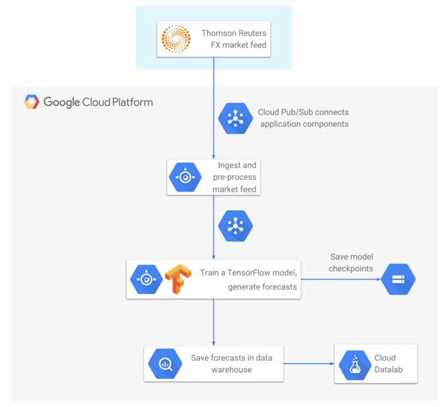
Cloud Pub/Sub: Connecting Application Components

Sending messages with Cloud Pub/Sub is easy. You initialize the Pub/Sub client, construct the message, and publish it:

The message payload can be in any format — JSON, protocol buffers, strings, etc. With one usage pattern, the publisher can specify the format and semantics of messages published on each topic. And this creates a de-facto semantic API, which is more lightweight and easier to maintain than a syntactic RPC-based API, since whenever you need to provide new functionality, no plumbing is required. With Cloud Pub/Sub, you only need to create a new topic for the new intended data format, and start publishing on it.

On the receiver side, you initialize the Cloud Pub/Sub client and repeatedly pull batches of messages. In the code snippet below, for example, each pull request retrieves a batch of up to 1000 messages. After a message is processed, the subscriber sends an acknowledgement, letting the system know that the message can now be safely garbage collected:

The status of published messages can be easily monitored with the Stackdriver tool, integrated with the Google Cloud Console. Stackdriver displays status metrics for each Cloud Pub/Sub topic and subscription owned by the project. The standard set of metrics includes the rate of published messages per second, average message size, message pulls per second, the number of undelivered messages, and the oldest unacknowledged (“unacked”) message.

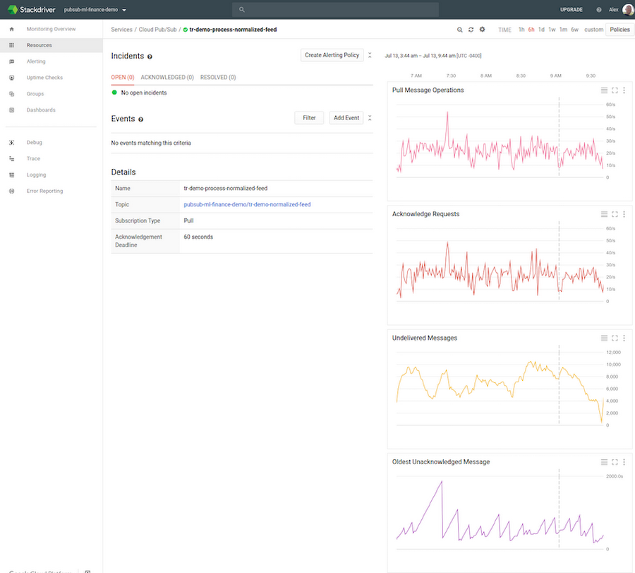
When deploying and configuring application components for the first time, Stackdriver is very helpful in verifying that subscribers are, for example, able to keep up with the publish load. If the number of undelivered messages and the age of the oldest unacked message keep increasing, the subscriber may need to be configured differently. For example, you may need more subscriber replicas, a higher CPU or memory allocation for each subscriber, or more efficient use of concurrency within the subscriber’s code.

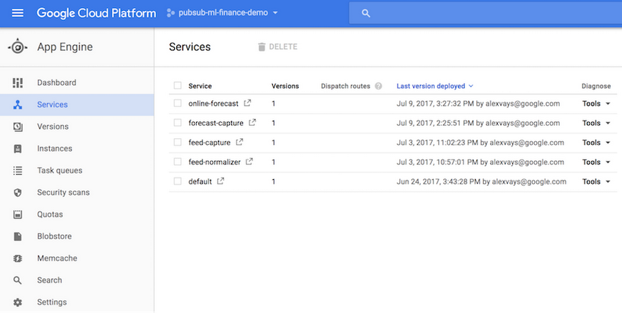
Next, we’ll look at how to deploy applications to run in Google Cloud using App Engine Flexible Environment. App Engine Flexible Environment runs Docker containers under the hood, so you get portability and flexibility, full integration into the Cloud Console, and convenient monitoring tools. You can easily see the status of deployed services and individual app instances:

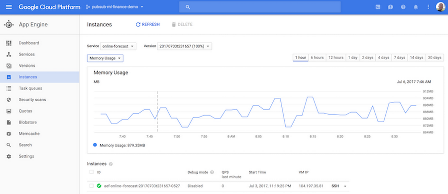
The dashboards provide access to various useful statistics, including historical memory usage and CPU usage for your application instances:

As an additional benefit, when deploying a new version of a service, App Engine does canarying, which means that it verifies that the new version runs reliably and doesn’t crash before switching over from the old version. For stateful applications expected to run under mostly continuous load, manual scaling is the optimal configuration option, as it doesn’t preempt the application during occasional periods of inactivity.

When an application runs within App Engine, it’s easy to display its internal state with a dynamically generated web page. The code snippet below shows an example of how to structure the forecast generating application when using Flask. The forecast generator class implements the main functionality — it creates several threads, receives market feed messages, trains the TensorFlow model, and so on. The app registers an HTTP endpoint and, when invoked, it calls the forecast generator to get its internal state, passes the state to a Jinja template, and renders the template to produce an HTML status page:

The next code snippet shows what the Jinja template for the forecast-generating application’s status page looks like. It’s basically HTML with embedded Python code:

When setting up an application to run in App Engine, the configuration requirements are specified in a deployment file in YAML format. The sample code snippet below shows that the application requires a Python runtime environment with manual scaling, running one service instance with 4 CPU cores and 12 GB of memory. The deployment file also specifies the environment variables that get passed to the application:

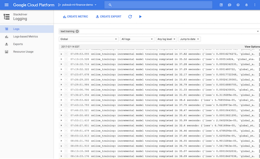
While on the topic of application monitoring, it’s good to mention Stackdriver Logging. It takes only a couple of lines of code to set up a cloud logger in your application, and one line to write a log message. You can then visually examine the logs from the Stackdriver dashboard, search for keywords, or export logs into a BigQuery table, Cloud Storage file, or a Pub/Sub topic for additional analysis:

Next, we’ll check out how to use TensorFlow to train a neural network and to generate real-time forecasts.

In this blog post we show how to train a TensorFlow model directly within App Engine. However, note that you can also train TensorFlow models using Google Cloud ML Engine. When using Cloud ML Engine, you get the additional benefits of automatic scaling and parallelization of TensorFlow model training.

TensorFlow provides interfaces at several abstraction levels. The lowest level classes can be used to build a neural network from scratch, using constants, variables, and operations. This interface provides most flexibility, but is also the most complex and time-consuming to use. The higher-level layers API implements standard types of layers used in the construction of neural networks, such as fully connected layers, convolutional layers, dropout layers, etc. Finally, the Estimators API provides highest-level abstractions, such as DNN Regressor and DNN Classifier. These classes are most effective to use when your problem can be solved with a standard neural network architecture.

In this blog post we show how to build a forecast-generating model using TensorFlow’s DNNRegressor class. The objective of the model is the following:

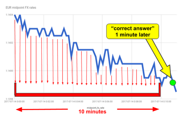
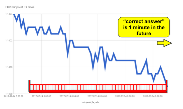
Given FX rates in the last 10 minutes, predict FX rate one minute later.

Each training example used in the model will include a 10-minute-long rolling window of observed FX rates from Thomson Reuters. With 1-second sampling frequency, a training example is represented as a 600-dimensional feature vector.

As the code snippet below illustrates, it takes just a few lines of code to set up a neural network. We specify the list of feature columns, the list of sizes of hidden fully connected layers, the name of the directory where TensorFlow will be saving model checkpoints, and the dropout rate. In this example, we’re using two hidden layers, with 10 nodes in each layer. The dropout rate specifies the probability that a neuron’s weight will be randomly zeroed out in a forward propagation pass during model’s training, as a way to make the model more resilient to noisy or dirty data. Note that when generating forecasts in serving, the dropout rate should always be set to zero:

Next, we’ll incrementally train and evaluate the DNNRegressor model, by repeatedly calling the fit() function. When invoked, it retrieves the next batch of training examples by calling the input function, and it trains the model for the specified number of training steps. In our forecasting application, each training example comprises a rolling window of FX rates as the model’s input, and the actual FX rate observed one minute later as the correct answer that the model will learn to predict:

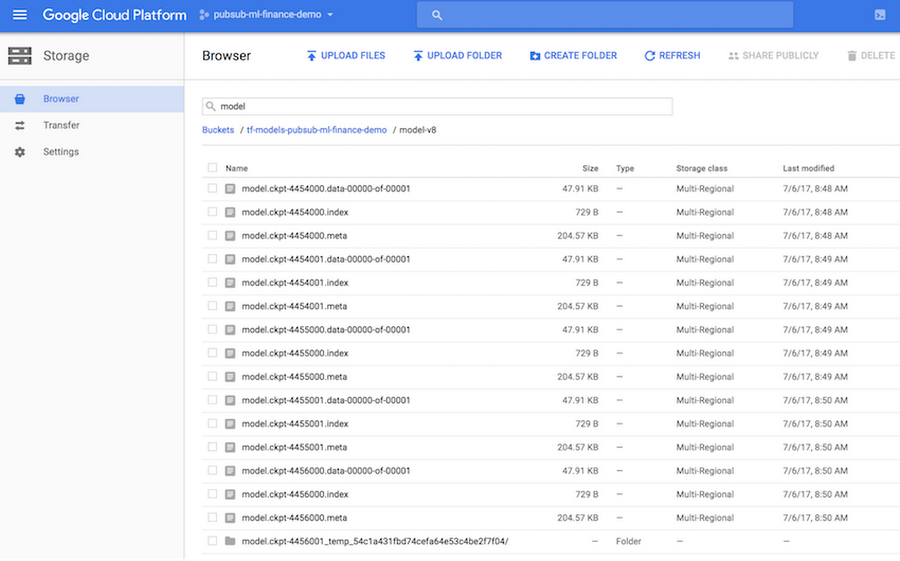
TensorFlow model snapshots (checkpoints) are automatically saved in the model directory specified when constructing the DNNRegressor object. The model directory can be either a regular file path or a Cloud Storage bucket path. The latter option enables your other applications deployed in Google Cloud to load saved checkpoints of trained TensorFlow models and use them to generate predictions or forecasts of FX rates. The screenshot below shows automatically saved model checkpoints in the Cloud Console (in this example, the Cloud Storage bucket path specified in the construction of DNNRegressor object was: gs://tf-models-demo/model-v8):

Finally, we want to generate our FX rate forecasts as model predictions. The predict_scores function retrieves the list of examples based on the latest 10-minute rolling window of FX rates, with one example per RIC (instrument identifier), and returns the predicted “correct answer” for each RIC, which by the model’s design is the forecasted FX rate at the 1-minute horizon:

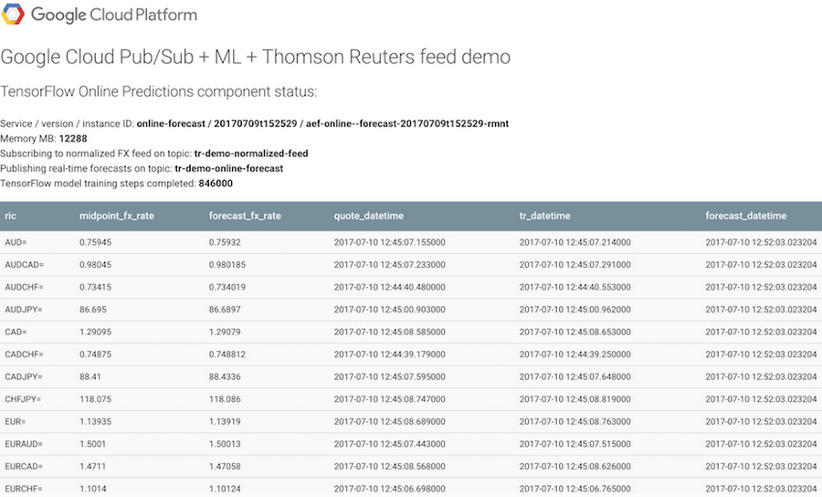
The screenshot below shows the App Engine-powered status page of our forecasting application. As described earlier in this post, the status page is generated dynamically, and upon each refresh it displays FX rates and forecast values updated in real time:

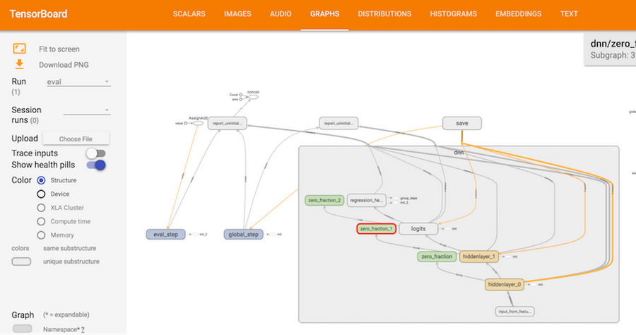
The neural network used to train the FX rate forecasting model can be visualized using TensorBoard. The screenshot below shows the internal structure of the DNNRegressor neural network used in our application. Using TensorBoard, we can look at each individual component in more detail, down to the low level of constants, variables, and operations:

In our example application, model predictions (FX rate forecasts) are generated in real time and shared with other apps in two ways: (1) the forecasts are published on a Cloud Pub/Sub topic, and (2) the forecasts are saved into BigQuery for warehousing and analysis.

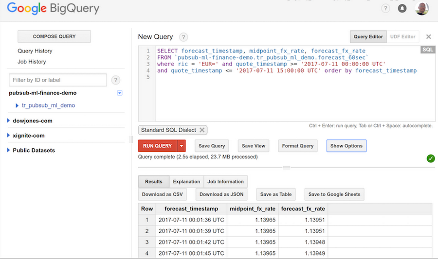
BigQuery is a fully managed data warehouse service with SQL support, designed for huge scale and parallelism in running queries on terabytes of data. FX rate forecasts saved into BigQuery can be easily retrieved and analyzed via the interactive BigQuery interface, as well as via APIs. The screenshot below illustrates how to run queries in the interactive mode:

Another useful tool is Datalab. It runs Jupyter notebooks that can combine text, python code, and output of the code, including graphics, charts and diagrams. Datalab can be used to retrieve our FX forecasts from BigQuery and to plot them in a graph. It only takes a few lines of Python code:

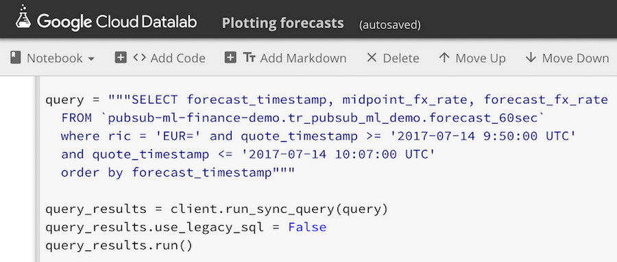
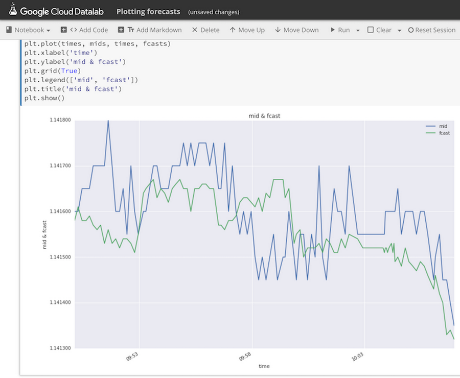
Query results can be plotted and visually examined directly in Datalab, so we can easily see forecasted FX rate values plotted next to observed FX midpoint rates published by Thomson Reuters:

To summarize, in this post we have shown how to train a machine learning model to predict FX rates using TensorFlow in Google Cloud, with application components running as App Engine services and communicating with each other by publishing messages via Cloud Pub/Sub and by writing data into BigQuery.

This blog post is accompanied by a talk presented by Alex (the author of this post) and Strategic Technology Partner Manager Annie Ma-Weaver at Google Cloud Summit New York 2017: