This article is the second part of a four-part series that discusses how you can predict customer lifetime value (CLV) by using AI Platform (AI Platform) on Google Cloud.
The articles in this series include the following:
- Part 1: Introduction. Introduces CLV and two modeling techniques for predicting CLV.
- Part 2: Training the model (this article). Discusses how to prepare the data and train the models.
- Part 3: Deploying to production. Describes how to deploy the models discussed in Part 2 to a production system.
- Part 4: Using AutoML Tables. Shows how to use AutoML Tables to build and deploy a model.
The code for implementing this system is in a GitHub repository. This series discusses what the code is for and how it's used.
Introduction
This article follows Part 1, in which you learned about two different models for predicting customer lifetime value (CLV):
- Probabilistic models
- Deep neural network (DNN) models, a type of machine learning model
As noted in Part 1, one of the goals of this series is to compare these models for predicting CLV. This part of the series describes how you can prepare the data and build and train both types of model to predict CLV, and provides some comparison information.
Installing the code
If you want to follow the process described in this article, you should install the sample code from GitHub.
If you have the gcloud CLI installed, open a terminal window on your computer to run these commands. If you don't have the gcloud CLI installed, open an instance of Cloud Shell.
Clone the sample code repository:
git clone
https://github.com/GoogleCloudPlatform/tensorflow-lifetime-value
Follow the installation instructions in the Install section of the README file to set up your environment.
Data preparation
This section describes how you can get the data and clean it.
Getting and cleaning the source dataset
Before you can calculate CLV, you must make sure that your source data contains at least the following:
- A customer ID that's used to differentiate individual customers.
- A purchase amount per customer that shows how much a customer spent at a specific time.
- A date for each purchase.
In this article, we discuss how to train models by using historical sales data from the publicly available Online Retail Data Set from the UCI Machine Learning Repository.[1]
The first step is to copy the dataset as a CSV file into
Cloud Storage.
Using one of the
loading tools for BigQuery,
you then create a table that's named data_source. (This name is arbitrary,
but the code in the GitHub repository uses this name.) The dataset is
available in a public bucket associated with this series and has already
been converted to CSV format.
- On your computer or in Cloud Shell, run the commands that are documented in the Setup section of the README file in the GitHub repository.
The example dataset contains the fields that are listed in the following
table. For the approach that we describe in this article, you use only the
fields where the Used column is set to Yes. Some fields are not
used directly, but help create new fields—for example, UnitPrice
and Quantity create order_value.
| Used | Field | Type | Description |
|---|---|---|---|
| No | InvoiceNo |
STRING |
Nominal. A 6-digit integral number uniquely assigned to each transaction.
If this code starts with letter c, it indicates a cancellation. |
| No | StockCode |
STRING |
Product (item) code. Nominal, a 5-digit integral number uniquely assigned to each distinct product. |
| No | Description |
STRING |
Product (item) name. Nominal. |
| Yes | Quantity |
INTEGER |
The quantities of each product (item) per transaction. Numeric. |
| Yes | InvoiceDate |
STRING |
Invoice Date and time in mm/dd/yy hh:mm format. The day and time when each transaction was generated. |
| Yes | UnitPrice |
FLOAT |
Unit price. Numeric. The product price per unit in sterling. |
| Yes | CustomerID |
STRING |
Customer number. Nominal. A 5-digit integral number uniquely assigned to each customer. |
| No | Country |
STRING |
Country name. Nominal. The name of the country where each customer resides. |
Cleaning the data
No matter which model you use, you must perform a set of preparation and cleaning steps that are common to all models. The following operations are required in order to get a set of workable fields and records:
- Group the orders by day instead of using
InvoiceNo, because the minimum time unit used by the probabilistic models in this solution is a day. - Keep only the fields that are useful for probabilistic models.
- Keep only records that have positive order quantities and monetary values, such as purchases.
- Keep only records with negative order quantities, such as returns.
- Keep only records with a customer ID.
- Keep only customers who bought something in the past 90 days.
- Keep only customers who bought at least twice in the time period that's being used to create features.
You can perform all of these operations using the following BigQuery query. (As with previous commands, you run this code wherever you cloned the GitHub repository.) Because the data is old, the date December 12, 2011, is considered today's date for purposes of this article.
This query performs two tasks. First, if the working dataset is large, the query shrinks it. (The working dataset for this solution is quite small, but this query can shrink an extremely large dataset by two orders of magnitude in a few seconds.)
Second, the query creates a base dataset to work on that looks like the following:
customer_id
|
order_date
|
order_value
|
order_qty_articles
|
|---|---|---|---|
| 16915 | 2011-08-04 | 173.7 | 6 |
| 15349 | 2011-07-04 | 107.7 | 77 |
| 14794 | 2011-03-30 | -33.9 | -2 |
The cleaned dataset also contains the order_qty_articles field. This field is
included only for use by the deep neural network (DNN) that's described in the
next section.
Defining the training and target intervals
To prepare for training the models, you must choose a threshold date. That date separates the orders into two partitions:
- Orders before the threshold date are used to train the model.
- Orders after the threshold date are used to compute the target value.

The Lifetimes library includes methods for preprocessing the data. However, the datasets that you use for CLV can be quite large, making it impractical to perform data preprocessing on a single machine. The approach described in this article uses queries that are executed directly in BigQuery to split orders into two sets. ML and probabilistic models use the same queries, ensuring that both models operate on the same data.
The optimal threshold date might differ for ML models and for probabilistic models. You can update this date value directly within the SQL statement. Think of the optimal threshold date as a hyperparameter. You find the most appropriate value by exploring the data and running some test trainings.
The threshold date is used in the WHERE clause of the SQL query that selects
training data from the cleaned data table, as shown in the following example:
Aggregating data
After you split the data into training and target intervals, you aggregate it to create actual features and targets for each customer. For probabilistic models, the aggregation is limited to recency, frequency, and monetary (RFM) fields. For DNN models, the models also use RFM features but can use additional features to make better predictions.
The following query shows how to create features for both DNN and probabilistic models at the same time:
The following table lists the features that are created by the query.
| Feature name | Description | Probabilistic | DNN |
|---|---|---|---|
monetary_dnn
|
The sum of all orders' monetary values per customer during the features period. | x | |
monetary_btyd
|
The average of all orders' monetary values for each customer during the features period. The probabilistic models assume that the value of the first order is 0. This is enforced by the query. | x | |
recency
|
The time between the first and last orders that were placed by a customer during the features period. | x | |
frequency_dnn
|
The number of orders placed by a customer during the features period. | x | |
frequency_btyd
|
The number of orders placed by a customer during the features period minus the first one. | x | |
T
|
The time between the first order placed by a customer and the end of the features period. | x | x |
time_between
|
The average time between orders for a customer during the features period. | x | |
avg_basket_value
|
The average monetary value of the customer's basket during the features period. | x | |
avg_basket_size
|
The number of items that the customer has on average in their basket during the features period. | x | |
cnt_returns
|
The number of orders that the customer has returned during the features period. | x | |
has_returned
|
Whether the customer has returned at least one order during the features period. | x | |
frequency_btyd_clipped
|
Same as frequency_btyd, but clipped by cap outliers. |
x | |
monetary_btyd_clipped
|
Same as monetary_btyd, but clipped by cap outliers. |
x | |
target_monetary_clipped
|
Same as target_monetary, but clipped by cap outliers. |
x | |
target_monetary
|
The total amount spent by a customer, including the training and target periods. | x |
The selection of these columns is done in the code. For the probabilistic models, selection is done using a Pandas DataFrame:
For the DNN models, TensorFlow features are defined in the
context.py file. For these models, the following are ignored as features:
customer_id. This is a unique value that is not useful as a feature.target_monetary. This is the target that the model must predict, and therefore not used as input.
Creating the training, evaluation, and test sets for DNN
This section applies only to the DNN models. To train an ML model, you should use three non-overlapping datasets:
The training (70–80%) dataset is used to learn weights to reduce a loss function. Training continues until the loss function no longer declines.
The evaluation (10–15%) dataset is used during the training phase to prevent overfitting, which is when a model performs well on training data but does not generalize well.
The test (10–15%) dataset should be used only once, after all training and evaluation has been completed, to perform a final measure of model performance. This dataset is one that the model has never seen during the training process, so it provides a statistically valid measure of model accuracy.
The following query creates a training set with about 70% of the data. The query segregates the data using the following technique:
- A hash of the customer ID is computed, which produces an integer.
- A modulo operation is used to select the hash values that are below a certain threshold.
The same concept is used for the evaluation set and test sets, where data that's above the threshold is kept.
Training
As you saw in the previous section, you can use different models to try to
predict CLV. The code that's used in this article was designed to let you decide
which model to use. You choose the model by using the model_type parameter
that you pass to the following training shell script. The code takes care of the
rest.
The first goal of the training is for both models to be able to beat a naive benchmark, which we define below. If both types of models can beat that (and they should), you can then compare how each type performs against the other.
Benchmarking the models
For purposes of this series, a naive benchmark is defined using the following parameters:
- Average basket value. This is calculated on all orders that are placed before the threshold date.
- Order count. This is calculated for the training interval on all orders that are placed before the threshold date.
- Count multiplier. This is calculated based on the ratio of the number of days before the threshold date and the number of days between the threshold date and now.
The benchmark naively assumes that the rate of purchases established by a customer during the training interval stays constant through the target interval. So if a customer bought 6 times over 40 days, the assumption is that they will buy 9 times over 60 days (60/40 * 6 = 9). Multiplying the count multiplier, the order count, and the average basket value for each customer gives a naive predicted target value for that customer.
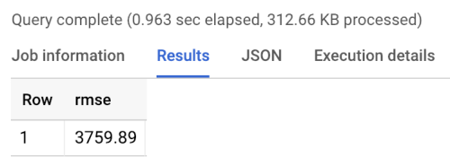
The benchmark error is the root mean square error (RMSE): the average across all customers of the absolute difference between the predicted target value and the actual target value. The RMSE is calculated using the following query in BigQuery:
The benchmark returns an RMSE of 3760, as shown in the following results of running the benchmark. Models should beat that value.
Probabilistic models
As mentioned in Part 1 of this series, this series uses a Python library called Lifetimes that supports various models including the Pareto/negative binomial distribution (NBD) and beta-geometric BG/NBD models. The following sample code shows how to use the Lifetimes library to perform lifetime value predictions with probabilistic models.
To generate CLV results by using the probabilistic model in your local
environment, you can run the following mltrain.sh script. You provide
parameters for the start and end dates of the training split and for the end of
the predict period.
./mltrain.sh local data --model_type paretonbd_model --threshold_date [YOUR_THRESHOLD_DATE] --predict_end [YOUR_END_DATE]
DNN models
The sample code includes implementations in TensorFlow of DNN using
the pre-made Estimator DNNRegressor class, as well as a custom Estimator
model. The DNNRegressor and the custom Estimator use the same number of
layers and number of neurons in each layer. Those values are hyperparameters
that need to be tuned. In the following task.py file, you can find a list
of some of the hyperparameters that were set to values that were tested
manually and gave good results.
If you're using AI Platform, you can use the hyperparameter tuning feature, which will test across a range of parameters that you define in a yaml file. AI Platform uses Bayesian optimization to search over the space of hyperparameters.
Results of comparing models
The following table shows the RMSE values for each model, as trained on the sample dataset. All models are trained on RFM data. RMSE values vary slightly between runs, due to random parameter initialization. The DNN model makes use of additional features such as average basket value and count of returns.
| Model | RMSE |
|---|---|
| DNN | 947.9 |
| BG/NBD | 1557 |
| Pareto/NBD | 1558 |
The results show that on this dataset, the DNN model outperforms the probabilistic models when predicting the monetary value. However, the relatively small size of the UCI dataset limits the statistical validity of these results. You should try each of the techniques on your dataset to see which gives you the best results. All models were trained by using the same original data (including customer ID, order date, and order value) on RFM values that were extracted from that data. The DNN training data included some additional features such as average basket size and count of returns.
The DNN model outputs only the overall customer monetary value. If you're interested in predicting frequency or churn, you must perform a few additional tasks:
- Prepare the data differently to change the target and possibly the threshold date.
- Retrain a regressor model to predict the target you're interested in.
- Tune the hyperparameters.
The intent here was to perform a comparison on the same input features between the two types of models. One advantage of using DNNs is that you might improve your results by adding more features than the ones used in this example. With DNNs, you could take advantage of data from sources such as clickstream events, user profiles, or product features.
Acknowledgements
Dua, D. and Karra Taniskidou, E. (2017). UCI Machine Learning Repository http://archive.ics.uci.edu/ml. Irvine, CA: University of California, School of Information and Computer Science.
What's next
- Read Part 3: Deploying to production of this series to understand how to deploy those models.
- Learn about other predictive forecasting solutions.
- Explore reference architectures, diagrams, and best practices about Google Cloud. Take a look at our Cloud Architecture Center.