BigQuery explained: Working with joins, nested & repeated data
Rajesh Thallam
Solutions Architect, Generative AI Solutions
In the previous post of BigQuery Explained series, we looked into querying datasets in BigQuery using SQL, how to save and share queries, a glimpse into managing standard and materialized views. In this post, we will focus on joins and data denormalization with nested and repeated fields. Let’s dive right into it!
Joins
Typically, data warehouse schemas follow a star or snowflake schema, where a centralized “fact” table containing events is surrounded by satellite tables called “dimensions” with the descriptive attributes related to the fact table. Fact tables are denormalized, and dimension tables are normalized. Star schema supports analytical queries in a data warehouse allowing to run simpler queries as the number of joins are limited, perform faster aggregations and improve query performance.
This is in contrast to an online transactional processing system (OLTP), where schema is highly normalized and joins are performed extensively to get the results. Most of the analytical queries in a data warehouse still require to perform JOIN operation to combine fact data with dimension attributes or with another fact table.
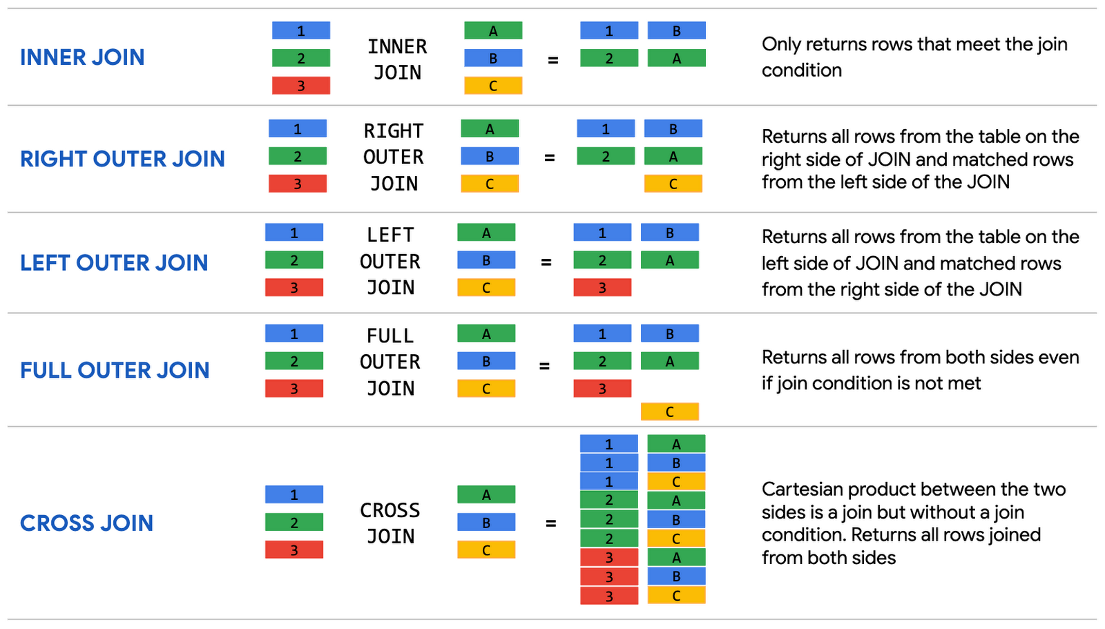
Let’s see how joins work in BigQuery. BigQuery supports ANSI SQL join types. JOIN operations are performed on two items based on join conditions and join type. Items in the JOIN operation can be BigQuery tables, subqueries, WITH statements, or ARRAYs (an ordered list with zero or more values of the same data type).
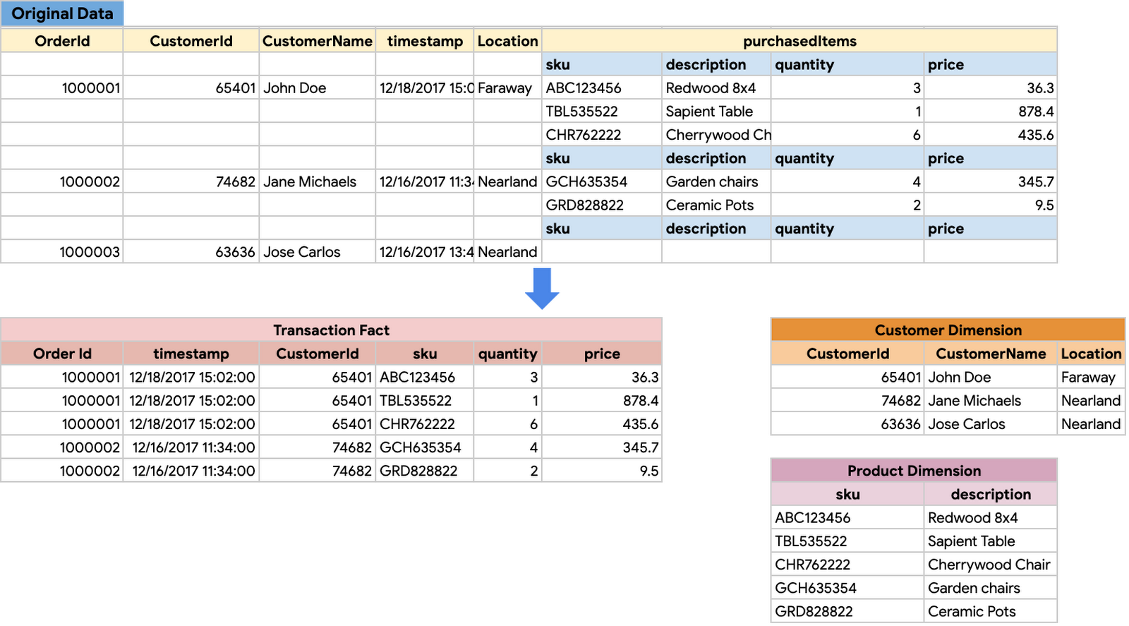
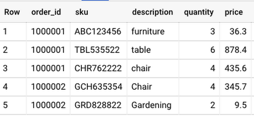
Let’s look at an example data warehouse schema for a retail store shown below. The original data table with retail transactions on the top is translated to a data warehouse schema with order details stored in a Transactions fact table and Product and Customer information as dimension tables.
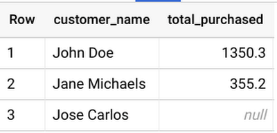
In order to find out how much each customer has spent in a given month, you would perform an OUTER JOIN between Transactions fact table with Customer dimension table to get the results. We will generate sample transactions and customer data on-the-fly using the WITH clause and see the JOIN in action. Run the below query:
Using WITH clause allows to name a subquery and use it in subsequent queries such as the SELECT statement here (also called Common Table Expressions). We use RIGHT OUTER JOIN between Customer and Transactions to get a list of all the customers with their total spend.
Note: The WITH clause is used primarily for readability because they are not materialized. If a query appears in more than one WITH clause, it executes in each clause.

Optimizing join patterns
Broadcast joins
When joining a large table to a small table, BigQuery creates a broadcast join where the small table is sent to each slot processing the large table.
Even though the SQL query optimizer can determine which table should be on which side of the join, it is recommended to order joined tables appropriately. The best practice is to place the largest table first, followed by the smallest, and then by decreasing size.
Hash joins
When joining two large tables, BigQuery uses hash and shuffle operations to shuffle the left and right tables so that the matching keys end up in the same slot to perform a local join. This is an expensive operation since the data needs to be moved.
In some cases, clustering may speed up hash joins. As mentioned in the previous post, clustering tends to colocate data in the same columnar files improving the overall efficiency of shuffling the data, particularly if there’s some pre-aggregation part of the query execution plan.
Self joins
In a self join, a table is joined with itself. This is typically a SQL anti-pattern which can be an expensive operation for large tables and might require to get data in more than one pass.
Instead, it is recommended to avoid self joins and instead use analytic (window) functions to reduce the bytes generated by the query.
Cross joins
Cross joins are a SQL anti-pattern and can cause significant performance issues as they generate larger output data than the inputs and in some cases queries may never finish.
To avoid performance issues with cross joins use aggregate functions to pre-aggregate the data or use analytic functions that are typically more performant than a cross join.
Skewed joins
Data skew can occur when the data in the table is partitioned into unequally sized partitions. When joining large tables that require shuffling data, the skew can lead to an extreme imbalance in the amount of data sent between the slots.
To avoid performance issues associated with skewed joins (or unbalanced joins), pre-filter data from the table as early as possible or split the query into two or more queries, if possible.
Refer to BigQuery best practices documentation for more such recommendations to optimize your query performance.
Denormalizing data with nested and repeated structures
When performing analytic operations on partially normalized schemas, such as star or snowflake schema in a data warehouse, multiple tables have to be joined to perform the required aggregations. However, JOINs are typically not as performant as denormalized structures. Query performance shows a much steeper decay in the presence of JOINs.
The conventional method of denormalizing data involves writing a fact, along with all its dimensions, into a flattened structure. In contrast, the preferred method for denormalizing data takes advantage of BigQuery’s native support for nested and repeated structures in JSON or Avro input data. Expressing records using nested and repeated structures can provide a more natural representation of the underlying data.
Continuing with the same data warehouse schema for a retail store, following are the key things to note:
An order in the
Transactionsbelongs to a singleCustomerandAn order in the
Transactionscan have multipleProduct(or items).
Earlier, we saw this schema organized into multiple tables. An alternative is to organize all of the information in a single table using nested and repeated fields.
A primer of nested and repeated fields
BigQuery supports loading nested and repeated data from source formats supporting object-based schemas, such as JSON, Avro, Firestore and Datastore export files. ARRAY and STRUCT or RECORD are complex data types to represent nested and repeated fields.
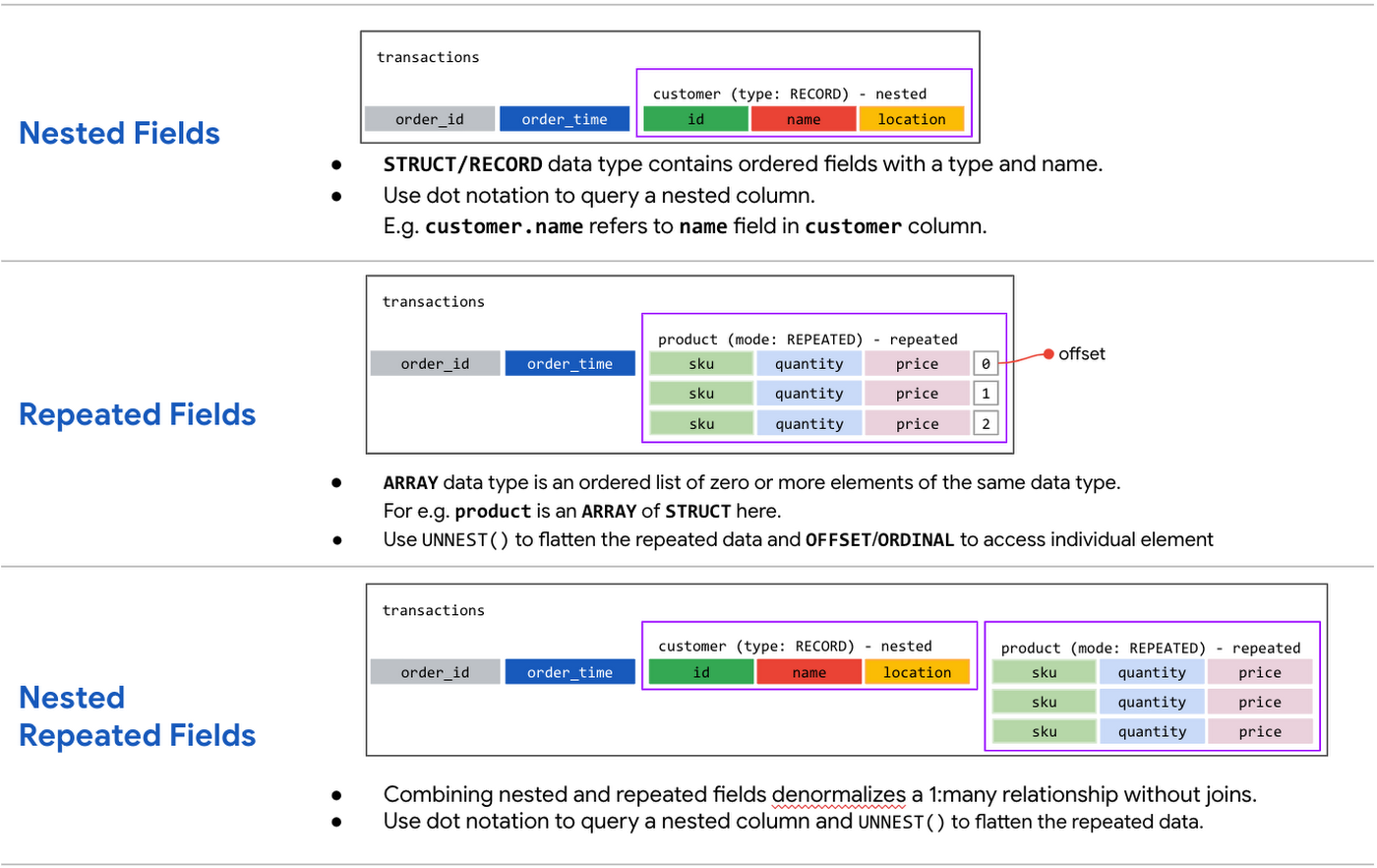
Nested Fields
A
STRUCTorRECORDcontains ordered fields each with a type and field name. You can define one or more of the child columns asSTRUCTtypes, referred to as nestedSTRUCTs (up to 15 levels of nesting).Let’s take
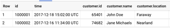
TransactionsandCustomerdata put into nested structure. Note that an order in theTransactionsbelongs to a singleCustomer. This can be represented as schema below:
Notice
customercolumn is of typeRECORDwith the ordered fields nested within the main schema along with Transactions fields—idandtime.BigQuery automatically flattens nested fields when querying. To query a column with nested data, each field must be identified in the context of the column that contains it. For example:
customer.idrefers to theidfield in thecustomercolumn.
Repeated Fields
An
ARRAYis an ordered list of zero or more elements of the same data type. An array of arrays is not supported. A repeated field adds an array of data inside a single field orRECORD.Let’s consider
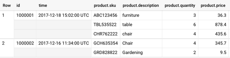
TransactionsandProductdata. An order in the Transactions can have multipleProduct(or items). When specifying the columnProductas repeated field in the schema, you would define the mode of theproductcolumn asREPEATED. The schema with repeated field is shown below:
Each entry in a repeated field is an
ARRAY. For example, each item in the product column for an order is of typeSTRUCTorRECORDwith sku, description, quantity andpricefields.BigQuery automatically groups data by “row” when querying one or more repeated fields.
To flatten the repeated (and grouped) data, you will use the UNNEST() function with the name of the repeated column. You can use UNNEST function only inside the FROM clause or IN operator.
Read more about handling ARRAYs and STRUCTs here.
Denormalized schema with nested repeated fields
Let’s put it all together and look at an alternate representation of theTransactions schema combining nested and repeated elements with Customer, and Product information in a single table. The schema is represented as follows: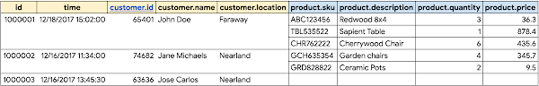
In the Transactions table, the outer part contains the order and customer information, and the inner part contains the line items of the order, which are represented as nested, repeated elements. Expressing records by using nested and repeated fields simplifies data load using JSON or Avro files. After you’ve created such a schema, you can perform SELECT, INSERT, UPDATE, and DELETE operations on any individual fields using a dot notation, for example, Order.sku.
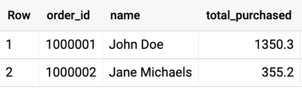
Transactions schema with nested and repeated fields to find total purchases on the order along with the customer name.Let’s unpack this query and understand how the data is denormalized.
Denormalized data representation
Transaction data is generated using a
WITHstatement, and each row consists oforderinformation,customerinformation, and a nested field containing individual items that are represented as anARRAYofSTRUCTs representing—sku,quantityandprice.Using
ARRAYofSTRUCTs, we gain significant performance advantage by avoiding tableJOINs.ARRAYofSTRUCTs can be treated as pre-joined tables retaining the structure of the data. Individual elements in the nested records can be retrieved only when needed . There is also the added benefit of having all the business context in one table, as opposed to managingJOINkeys and associated tables.
Normalizing data for analyzing
In the
SELECTquery, we read fields such aspricefrom the nested record usingUNNEST()function and dot notation. For example orders.priceUNNEST()helps to bring the array elements back into rowsUNNEST()always follows the table name in theFROMclause (conceptually like a pre-joined table)
Running the query above returns results with order, customer, and total order amount.
Guidelines for designing a denormalized schema
Following are general guidelines for designing a denormalized schema in BigQuery:
Denormalize a dimension table larger than 10GB, unless there is strong evidence that the costs of data manipulation, such as
UPDATEandDELETEoperations, outweigh the benefits of optimal queries.Keep a dimension table smaller than 10GB normalized, unless the table rarely goes through
UPDATEandDELETEoperations.Take full advantage of nested and repeated fields in denormalized tables.
Refer to this article for more on denormalization and designing schema in a data warehouse.
What Next?
In this post, we worked with joins, reviewed optimizing join patterns and denormalized data with nested and repeated fields.
Working with JOIN in BigQuery
Working with Analytic (window) functions in BigQuery
Working with Nested and repeated data in BigQuery [Video] [Docs]
BigQuery best practices for query performance including joins and more
Querying a public dataset in BigQuery with nested and repeated fields on your BigQuery Sandbox — Thanks to Evan Jones for the demo! (Codelab coming soon!)
In the next post, we will see data manipulation in BigQuery along with scripting, stored procedures and more.
Stay tuned. Thank you for reading! Have a question or want to chat? Find me on Twitter or LinkedIn.
The complete BigQuery Explained series
- BigQuery explained: An overview of BigQuery's architecture
- BigQuery explained: Storage overview, and how to partition and cluster your data for optimal performance
- BigQuery explained: How to ingest data into BigQuery so you can analyze it
- BigQuery explained: How to query your data
- BigQuery explained: Working with joins, nested & repeated data
- BigQuery explained: How to run data manipulation statements to add, modify and delete data stored in BigQuery