After Lambda: Exactly-once processing in Cloud Dataflow, Part 2 (Ensuring low latency)
Reuven Lax
Software Engineer
In Part 1 of this series, you learned what “exactly-once” processing means in the context of Google Cloud Dataflow, and how its streaming shuffle can implement that guarantee. We also described a technique where a catalog of record ids is stored in each receiver key. To reiterate: For every record that arrives, Cloud Dataflow looks up the catalog of ids already seen to determine whether this record is a duplicate. Every output from step to step is checkpointed to storage to ensure the generated record ids are stable.
However, unless implemented carefully, this process would significantly degrade pipeline performance for customers by creating a huge increase in reads and writes. Thus, for exactly-once processing to be viable for Cloud Dataflow customers (if not contributory to additional stream-processing use cases), that IO has to be reduced, in particular by preventing IO on every record.
In this post, you’ll learn how Cloud Dataflow achieves this goal via two key techniques: graph optimization and Bloom filters.
Graph optimizations
The Cloud Dataflow service runs a series of optimizations on the pipeline graph before executing it. One such optimization is fusion, in which the service fuses many logical steps into a single execution stage.The following diagram shows some simple examples: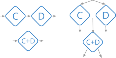
All fused steps are run as an in-process unit so there’s no need to store exactly-once data for each of them. In many cases, fusion reduces the entire graph down to a few steps, greatly reducing the amount of data transfer needed (and saving on state usage as well).
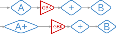
Cloud Dataflow also optimizes Combine operations (such as Count and Sum) by performing partial combining locally before sending the data to the main grouping operation. This approach can greatly reduce the number of messages for delivery, consequently also reducing the number of reads and writes.
Bloom filters
The optimizations above are general techniques that improve exactly-once performance as a byproduct. For an optimization aimed strictly at improving exactly-once processing, we turn to Bloom filters.In a healthy pipeline most arriving records will not be duplicates. We can use that fact to greatly improve performance via Bloom filters, which are compact data structures that allow for quick set-membership checks. Bloom filters have a very interesting property: they can return false positives but never false negatives. If the filter says “Yes, the element is in the set,” we know that the element is probably in the set (and the probability can be calculated). However, if the filter says an element is not in the set, then it definitely isn’t. This function is a perfect fit for the task at hand.
The implementation in Cloud Dataflow works like this: Each worker keeps a Bloom filter of every identifier it has seen. Whenever a new record id shows up, it looks it up in the filter. If the filter returns false, then this record is not a duplicate and the worker can skip the more expensive lookup from stable storage. It only has to do that second lookup if the Bloom filter returns true, but as long as the filter’s false-positive rate is low that step is rarely needed.
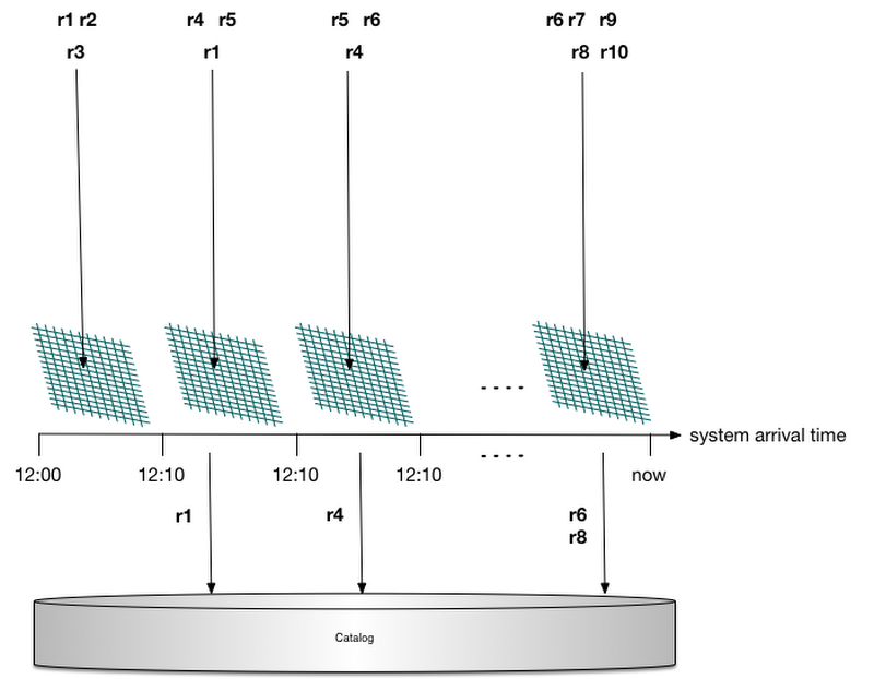
Bloom filters tend to fill up over time, however, and as that happens, the false-positive rate increases. We also need to construct this Bloom filter anew when a worker restarts by scanning the id catalog stored in state. Helpfully, Cloud Dataflow attaches a system timestamp to each record. (Note: these are not the custom user-supplied timestamps used for windowing but rather deterministic processing-time timestamps that are applied by the sending worker.) Thus instead of creating a single Bloom filter, the service creates a separate one for every 10-minute range. When a record arrives, Cloud Dataflow picks the appropriate filter to check based on the system timestamp. This step prevents the Bloom filters from saturating as filters get garbage-collected, and also bounds the amount of data that needs to be scanned at startup.
This process is illustrated in the below diagram: Records arrive in the system and are delegated to a Bloom filter based on their arrival time. None of the records hitting the first filter are duplicates, and all their catalog lookups are filtered. Record r1 is delivered a second time, so a catalog lookup is needed to verify that it is indeed a duplicate; the same is true for records r4 and r6. Record r8 is not a duplicate; however, due to a false positive in its Bloom filter, a catalog lookup is generated (which will determine that r8 is not a duplicate and should be processed).
Garbage collection
Every Cloud Dataflow worker persistently stores a catalog of unique record identifiers it has seen. As Cloud Dataflow’s state and consistency model is per-key, in reality each key stores a catalog of records that have been delivered to that key. We can’t store these identifiers forever, or all available storage will eventually fill up. To avoid that issue, garbage collection of acknowledged record ids is needed.One strategy for accomplishing this goal would be for senders to tag each record with a strictly-increasing sequence number in order to track the earliest sequence number still in flight (corresponding to an unacknowledged record delivery). Any identifier in the catalog with an earlier sequence number could then be garbage-collected, since all earlier records have already been acknowledged.
There is a better alternative, however. As previously mentioned, Cloud Dataflow already tags each record with a system timestamp that is used for bucketing exactly-once Bloom filters. Consequently, instead of using sequence numbers to garbage-collect the exactly-once catalog, Cloud Dataflow calculates a garbage-collection watermark based on these system timestamps.
A nice side benefit of this approach is that since this watermark is based on the amount of physical time spent waiting in a given stage (unlike the data watermark, which is based on custom event times), it provides intuition on what parts of the pipeline are slow. This metadata is the basis for the System Lag metric shown in the Cloud Dataflow UI.
What happens if a record arrives with an old timestamp and we’ve already garbage-collected identifiers for this time? This can happen due to an effect we call network remnants, in which an old message gets stuck for an indefinite period of time inside the network and then suddenly shows up. Well, the low watermark that triggers garbage collection won’t advance until record deliveries have been acknowledged, so we know that this record has already been successfully processed. Such network remnants are clearly duplicates and are ignored.
Next steps
Ideally, you’ve now learned how exactly-once data processing, which was once thought to be incompatible with low-latency results, is not only possible in Cloud Dataflow but efficient. This unlocks a rich set of use cases for streaming where exactly-once processing is critical. Pipelines that produce business-critical metrics will produce correct results and do so with low latency. No longer do you need to periodically run a “fixup” batch pipeline to produce accurate results.In the next post, we’ll dive deeper into how to write correct sources and sinks that preserve exactly-once semantics.