AI in depth: monitoring home appliances from power readings with ML

As the popularity of home automation and the cost of electricity grow around the world, energy conservation has become a higher priority for many consumers. With a number of smart meter devices available for your home, you can now measure and record overall household power draw, and then with the output of a machine learning model, accurately predict  individual appliance behavior simply by analyzing meter data. For example, your electric utility provider might send you a message if it can reasonably assess that you left your refrigerator door open, or if the irrigation system suddenly came on at an odd time of day.

In this post, you’ll learn how to accurately identify home appliances’ (e.g. electric kettles and washing machines, in this dataset) operating status using smart power readings, together with modern machine learning techniques such as long short-term memory (LSTM) models. Once the algorithm identifies an appliance’s operating status, we can then build out a few more applications. For example:

• Anomaly detection: Usually the TV is turned off when there is no one at home. An application can send a message to the user if the TV turns on at an unexpected or unusual time.
• Habit-improving recommendations: We can present users the usage patterns of home appliances in the neighborhood at an aggregated level so that they can compare or refer to the usage patterns and optimize the usage of their home appliances.

We developed our end-to-end demo system entirely on Google Cloud Platform, including data collection through Cloud IoT Core, a machine learning model built using TensorFlow and trained on Cloud Machine Learning Engine, and real-time serving and prediction made possible by Cloud Pub/Sub, App Engine and Cloud ML Engine. As you progress through this post, you can access the full set of source files in the GitHub repository here.

Introduction

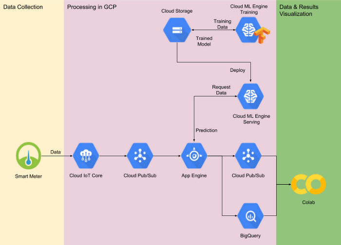
The growing popularity of IoT devices and the evolution of machine learning technologies have brought new opportunities for businesses. In this post, you’ll learn how home appliances’ (for example, an electric kettle and a washing machine) operating status (on/off) can be inferred from gross power readings collected by a smart meter, together with state-of-the-art machine learning techniques. An end-to-end demo system, developed entirely on Google Cloud Platform (as shown in Fig. 1), includes:

• Data collection and ingest through Cloud IoT Core and Cloud Pub/Sub
• A machine learning model, trained using Cloud ML Engine
• That same machine learning model, served using Cloud ML Engine together with App Engine as a front end
• Data visualization and exploration using BigQuery and Colab

The animation below shows real-time monitoring, as real-world energy usage data is ingested through Cloud IoT Core into Colab.

IoT extends the reach of machine learning

Data ingestion

In order to train any machine learning model, you need data that is both suitable and sufficient in quantity. In the field of IoT, we need to address a number of challenges in order to reliably and safely send the data collected by smart IoT devices to remote centralized servers. You’ll need to consider data security, transmission reliability, and use case-dependent timeliness, among other factors.

Cloud IoT Core is a fully managed service that allows you to easily and securely connect, manage, and ingest data from millions of globally dispersed devices. The two main features of Cloud IoT Core are its device manager and its protocol bridge. The former allows you to configure and manage individual devices in a coarse-grained way by establishing and maintaining devices’ identities along with authentication after each connection. The device manager also stores each device’s logical configuration and is able to remotely control the devices—for example, changing a fleet of smart power meters’ data sampling rates. The protocol bridge provides connection endpoints with automatic load balancing for all device connections, and natively supports secure connection over industry standard protocols such as MQTT and HTTP. The protocol bridge publishes all device telemetry to Cloud Pub/Sub, which can then be consumed by downstream analytic systems. We adopted the MQTT bridge in our demo system and the following code snippet includes MQTT-specific logic.

Data consumption

After the system publishes data to Cloud Pub/Sub, it delivers a message request to the “push endpoint,” typically the gateway service that consumes the data. In our demo system, Cloud Pub/Sub pushes data to a gateway service hosted in App Engine which then forwards the data to the machine learning model hosted in the Cloud ML Engine for inference, and at the same time stores the raw data together with received prediction results in BigQuery for later (batch) analysis.

While there are numerous business-dependent use cases you can deploy based on our sample code, we illustrate raw data and prediction results visualization in our demo system. In the code repository, we have provided two notebooks:

• EnergyDisaggregationDemo_Client.ipynb: this notebook simulates multiple smart meters by reading in power consumption data from a real world dataset and sends the readings to the server. All Cloud IoT Core-related code resides in this notebook.
• EnergyDisaggregationDemo_View.ipynb: this notebook allows you to view raw power consumption data from a specified smart meter and our model's prediction results in almost real time.

If you follow the deployment instructions in the README file and in the accompanying notebooks, you should be able to reproduce the results shown in Figure 2. Meanwhile, if you’d prefer to build out your disaggregation pipeline in a different manner, you can also use Cloud Dataflow and Pub/Sub I/O to build an app with similar functionality.

Data processing and machine learning

Dataset introduction and exploration

We trained our model to predict each appliance’s on/off status from gross power readings, using the UK Domestic Appliance-Level Electricity (UK-DALE, publicly available here¹) dataset  in order for this end-to-end demo system to be reproducible. UK-DALE records both whole-house power consumption and usage from each individual appliance every 6 seconds from 5 households. We demonstrate our solution using the data from house #2, for which the dataset includes a total of 18 appliances’ power consumption. Given the granularity of the dataset (a sample rate of ⅙ Hz), it is difficult to estimate appliances with relatively tiny power usage. As a result, appliances such as laptops and computer monitors are removed from this demo. Based on a data exploration study shown below, we selected eight appliances out of the original 18 items as our target appliances: a treadmill, washing machine, dishwasher, microwave, toaster, electric kettle, rice cooker and “cooker,” a.k.a., electric stovetop.

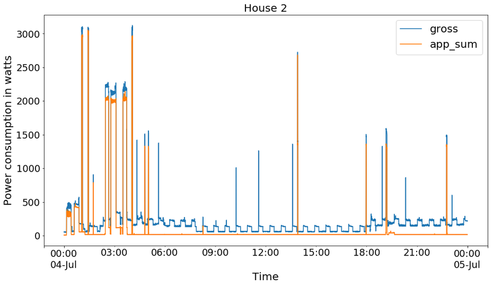
The figure below shows the power consumption histograms of selected appliances. Since all the appliances are off most of the time, most of the readings are near zero. Fig. 4 shows the comparisons between aggregate power consumption of selected appliances (`app_sum`) and the whole-house power consumption (`gross`). It is worth noting that the input to our demo system is the gross consumption (the blue curve) because this is the most readily available power usage data, and is even measurable outside the home.

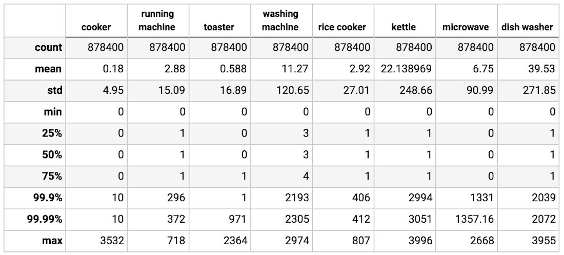
The data for House #2 spans from late February to early October 2013. We used data from June to the end of September in our demo system due to missing data at both ends of the period. The descriptive summary of selected appliances is illustrated in Table 1. As expected, the data is extremely imbalanced in terms of both “on” vs. “off” for each appliance and power consumption scale of each appliance, which introduces the main difficulty of our prediction task.

Preprocessing the data

Since UK-DALE did not record individual appliance on/off status, one key preprocessing step is to label the on/off status of each appliance at each timestamp. We assume an appliance to be “on” if its power consumption is larger than one standard deviation from the sample mean of its power readings, given the fact that appliances are off most of the time and hence most of the readings are near zero. The code for data preprocessing can be found in the notebook provided, and you can also download the processed data from here.

With the preprocessed data in CSV format, TensorFlow’s Dataset class serves as a convenient tool for data loading and transformation—for example, the input pipeline for machine learning model training. For example, in the following code snippet lines 7 - 9 load data from the specified CSV file and lines 11 - 13 transform data into our desired time-series sequence.

In order to address the data imbalance issue, you can either down-sample the majority class or up-sample the minority class. In our case, we propose a probabilistic negative down-sampling method: we’ll preserve the subsequences in which at least one appliance remains on, but we’ll filter the subsequences with all appliances off, based on a certain probability and threshold. The filtering logic integrates easily with the tf.data API, as in the following code snippet:

Finally, you’ll want to follow best practices from Input Pipeline Performance Guide to ensure that your GPU or TPU (if they are used to speed up training process) resources are not wasted while waiting for the data to load from the input pipeline. To maximize usage, we employ parallel mapping to parallelize data transformation and prefetch data to overlap the preprocessing and model execution of a training step, as shown in the following code snippet:

The machine learning model

We adopt a long short-term memory (LSTM) based network as our classification model. Please see Understanding LSTM Networks for an introduction to recurrent neural networks and LSTMs. Fig. 5 depicts our model design, in which an input sequence of length n is fed into a multilayered LSTM network, and prediction is made for all m appliances. A dropout layer is added for the input of LSTM cell, and the output of the whole sequence is fed into a fully connected layer. We implemented this model as a TensorFlow estimator.

There are two ways of implementing the above architecture: TensorFlow native API (tf.layers and tf.nn) and Keras API (tf.keras). Compared to TensorFlow’s native API, Keras serves as a higher level API that lets you train and serve deep learning models with three key advantages: ease of use, modularity, and extensibility. tf.keras is TensorFlow's implementation of the Keras API specification. In the following code sample, we implemented the same LSTM-based classification model using both methods, so that you can compare the two:

Model authoring using TensorFlow’s native API:

Model authoring using the Keras API:

Training and hyperparameter tuning

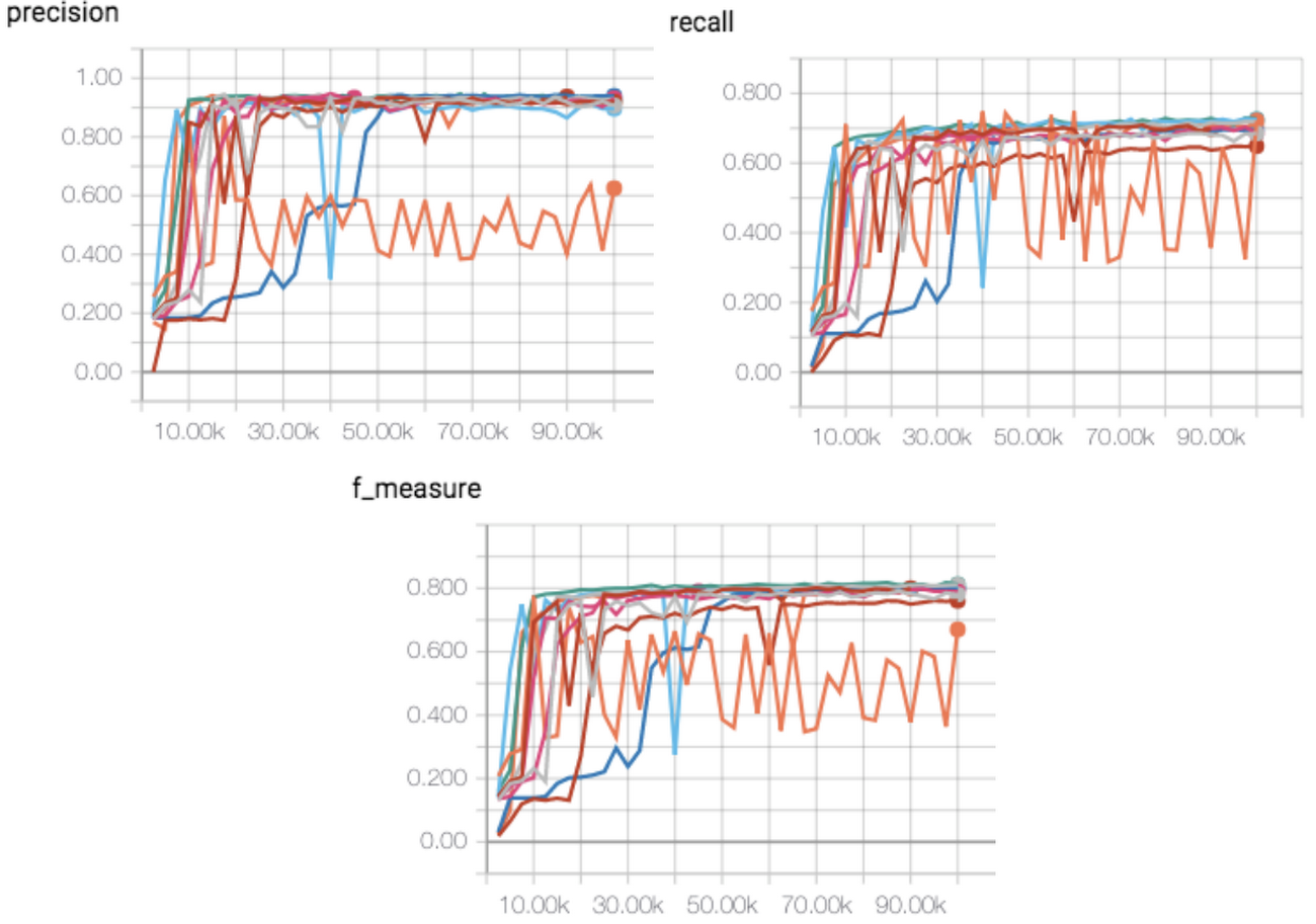
Cloud Machine Learning Engine supports both training and hyperparameter tuning. Figure 6 shows the average (over all appliances) precision, recall and f_score for multiple trials with different combinations of hyperparameters. We observed that hyperparameter tuning significantly improves model performance.

We selected two experiments with optimal scores from hyperparameter tunings and report their performances in Table 2.

Table 3 lists the precision and recall of each individual appliance. As mentioned in the previous “Dataset introduction and exploration” section, the cooker and the treadmill (“running machine”) are difficult to predict, because their peak power consumptions were significantly lower than other appliances.

Conclusion

We have provided an end-to-end demonstration of how you can use machine learning to determine the operating status of home appliances accurately, based on only smart power readings. Several products including Cloud IoT Core,  Cloud Pub/Sub,  Cloud ML Engine, App Engine and BigQuery are orchestrated to support the whole system, in which each product solves a specific problem required to implement this demo, such as data collection/ingestion, machine learning model training, real time serving/prediction, etc. Both our code and data are available for those of you who would like to try out the system for yourself.

We are optimistic that both we and our customers will develop ever more interesting applications at the intersection of more capable IoT devices and fast-evolving machine learning algorithms. Google Cloud provides both the IoT infrastructure and machine learning training and serving capabilities that make newly capable smart IoT deployments both a possibility and a reality.

_{1. Jack Kelly and William Knottenbelt. The UK-DALE dataset, domestic appliance-level electricity demand and whole-house demand from five UK homes. Scientific Data 2, Article number:150007, 2015, DOI:10.1038/sdata.2015.7.}