Clouds in the cloud: Weather forecasting in Google Cloud

Weather forecasting and climate modeling are two of the world's most computationally complex and demanding tasks. Further, they’re extremely time-sensitive and in high demand — everyone from weekend travelers to large-scale industrial farming operators wants up-to-date weather predictions. To provide timely and meaningful predictions, weather forecasters usually rely on high performance computing (HPC) clusters hosted in an on-premises data center. These on-prem HPC systems require significant capital investment and have high long-term operational costs. They consume a lot of electricity, have largely fixed configurations, and the underlying computer hardware is replaced infrequently. 

Using the cloud instead offers increased flexibility, constantly refreshed hardware, high reliability, geo-distributed compute and networking, and a “pay for what you use” pricing model. Ultimately, cloud computing allows forecasters and climate modelers to provide timely and accurate results on a flexible platform using the latest hardware and software systems, in a cost effective manner. This is a big shift compared with traditional approaches to weather forecasting, and can appear challenging. To help, weather forecasters can now run the Weather Research and Forecasting (WRF) modeling system easily on Google Cloud using the new WRF VM image from Fluid Numerics, and achieve the performance of an on-premises supercomputer for a fraction of the price. With this solution, weather forecasters can get a WRF simulation up and running on Google Cloud in less than an hour!

A closer look at WRF

Weather Research and Forecasting (WRF) is a popular open-source numerical weather prediction modeling system used by both researchers and operational organizations. While WRF is primarily used for weather and climate simulation, teams have extended it to support interactions with chemistry, forest fire modeling, and other use cases. WRF development began in the late 1990s through a collaboration between the National Center for Atmospheric Research (NCAR), National Oceanic and Atmospheric Administration (NOAA), U.S. Air Force, Naval Research Laboratory, University of Oklahoma, and the Federal Aviation Administration. The WRF community comprises more than 48,000 users spanning over 160 countries, with the shared goal of supporting atmospheric research and operational forecasting.

The Google Cloud WRF image is built using Google's MPI best practices for HPC, with the exception that hyperthreading is not disabled by default, and is easily integrated with other HPC solutions on Google Cloud, including SchedMD’s Slurm-GCP. Normally, installing WRF and its dependencies is a time consuming process. With these new WRF VM images, deploying a scalable HPC cluster with WRF v4.2 pre-installed is quick and easy with our Codelab. OpenMPI 4.0.2 was used throughout this work. Google has had good success with Intel MPI, and we intend to study whether further performance gains can be achieved in this context.

Optimizing WRF

Determining the optimal architecture and build settings for performance and cost was a key part of the process in developing the WRF images. We evaluated how to select the ideal compiler, right CPU platform, and the best file system for handling file IO, so you don't have to. As a test case for assessing performance, we used the CONUS 2.5km benchmark. 

Below, the CONUS 2.5km runtime and cost figure shows the run time required for simulating WRF over a two-hour forecast using 480 MPI ranks (a way of numbering processes) for different machine types available on Google Cloud. For each machine type, we’re showing the lowest measured run time from a suite of tests that varied compiler, compiler optimizations, and task affinity.

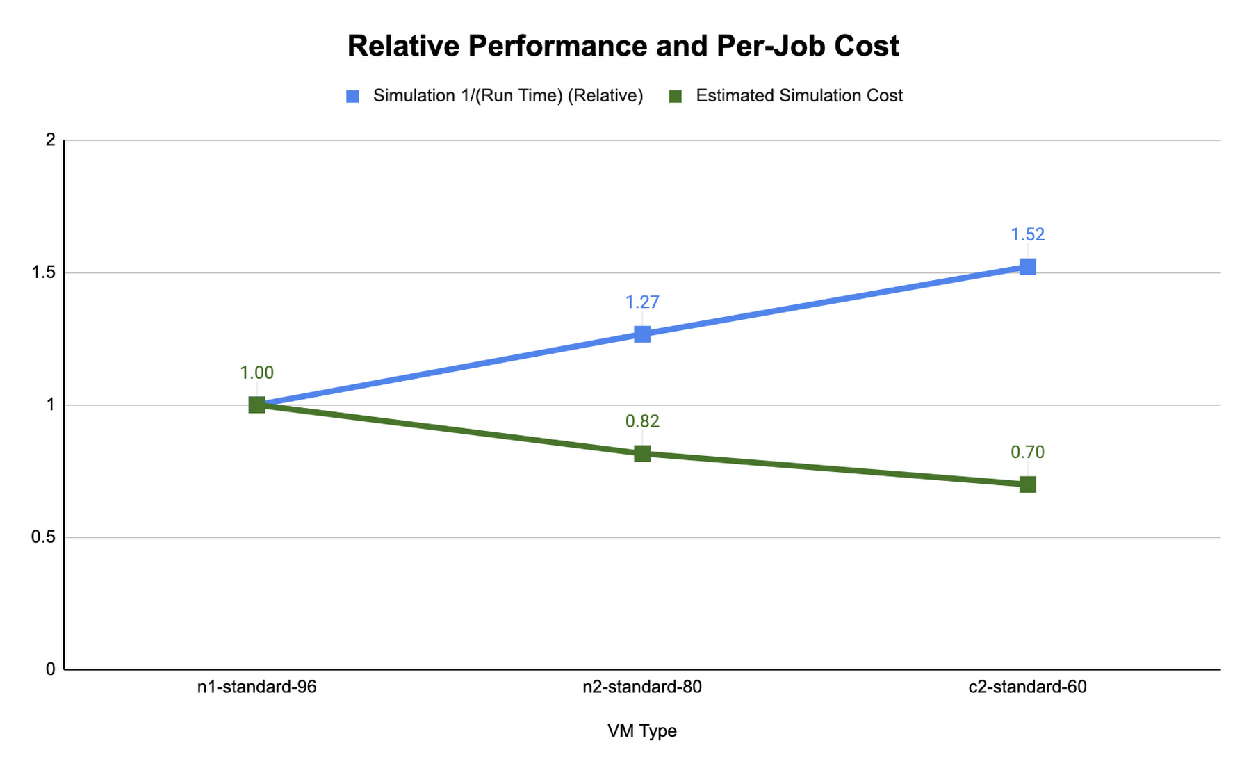
We found that compute-optimized c2 instances provided the shortest run time. The Slurm job scheduler allows you to map the MPI tasks to compute hardware using task affinity flags. When optimizing the runtime and cost for each machine type, we compared using srun –map-by core –bind-to core to launch WRF, which maps each MPI process to a physical core (two vCPU per MPI rank), and srun –map-by thread –bind-to thread, which maps each MPI process to a single vCPU. Mapping by core and binding MPI ranks to cores is akin to disabling hyperthreading.

The ideal simulation cost and runtime for CONUS 2.5km for each platform is found when each MPI rank is subscribed to each vCPU. When binding to vCPUs, half as many compute resources are needed when compared to binding to physical cores lowering the per-second cost for the simulation. For CONUS 2.5km, we also found that although mapping MPI ranks to cores results in reduced runtime for the same number of MPI ranks, the performance gains are not significant enough to outweigh the cost savings. For this reason, the WRF-GCP solution does not disable hyperthreading by default.

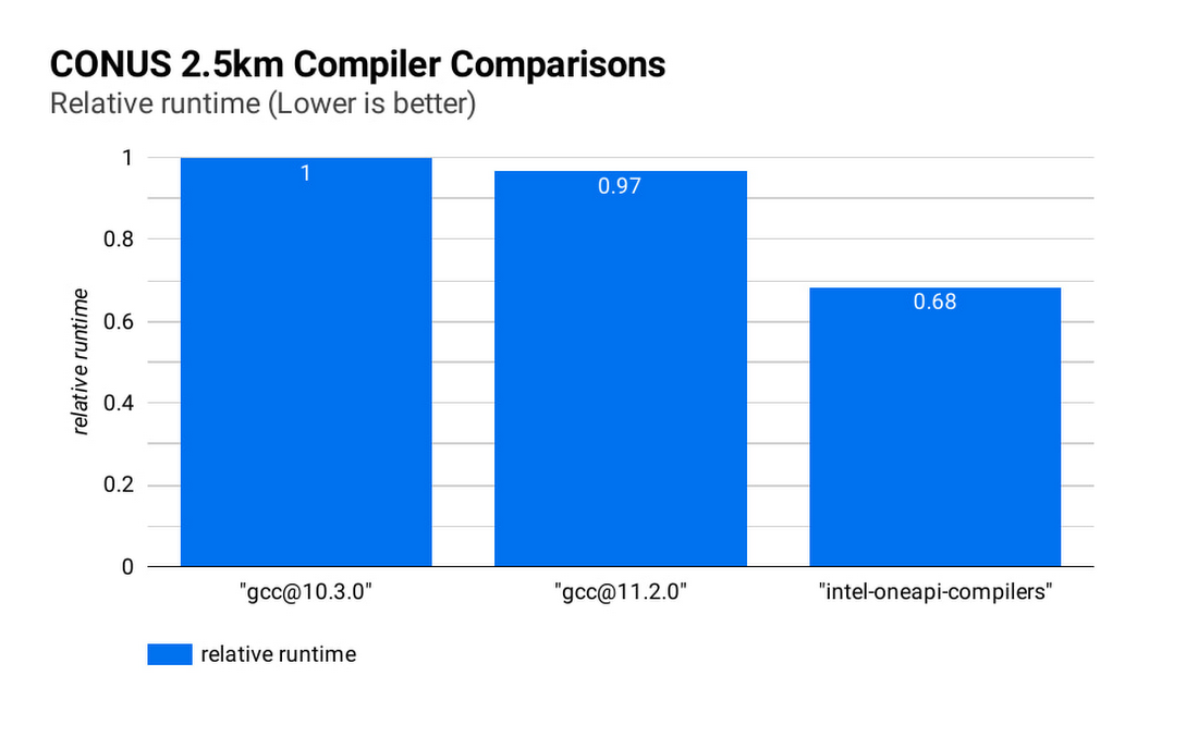
Runtime and simulation cost can be further reduced by selecting an ideal compiler: the figure below (CONUS 2.5km Compiler Comparisons) shows the simulation runtime for the WRF CONUS 2.5km benchmark on eight c2-standard-60 instances, using GCC 10.30, GCC 11.2.0 and the Intel® OneAPI® compilers (v2021.2.0). In all cases, WRF is built using level 3 compiler optimizations and Cascade Lake target architecture flags. By compiling WRF with the Intel® OneAPI® compilers, the WRF simulation runs about 47% faster than the GCC builds, and at about 68% of the cost, on the same hardware. We’ve used OpenMPI 4.0.2 with each of the compilers as the MPI implementation in this work. With other applications, Google has seen good performance with Intel MPI 2018, and we intend to investigate performance comparisons with this and other MPI implementations.

File IO in WRF can become a significant bottleneck as the number of MPI ranks increases. Obtaining the optimal file IO performance requires using parallel file IO in WRF and leveraging a parallel file system such as Lustre.

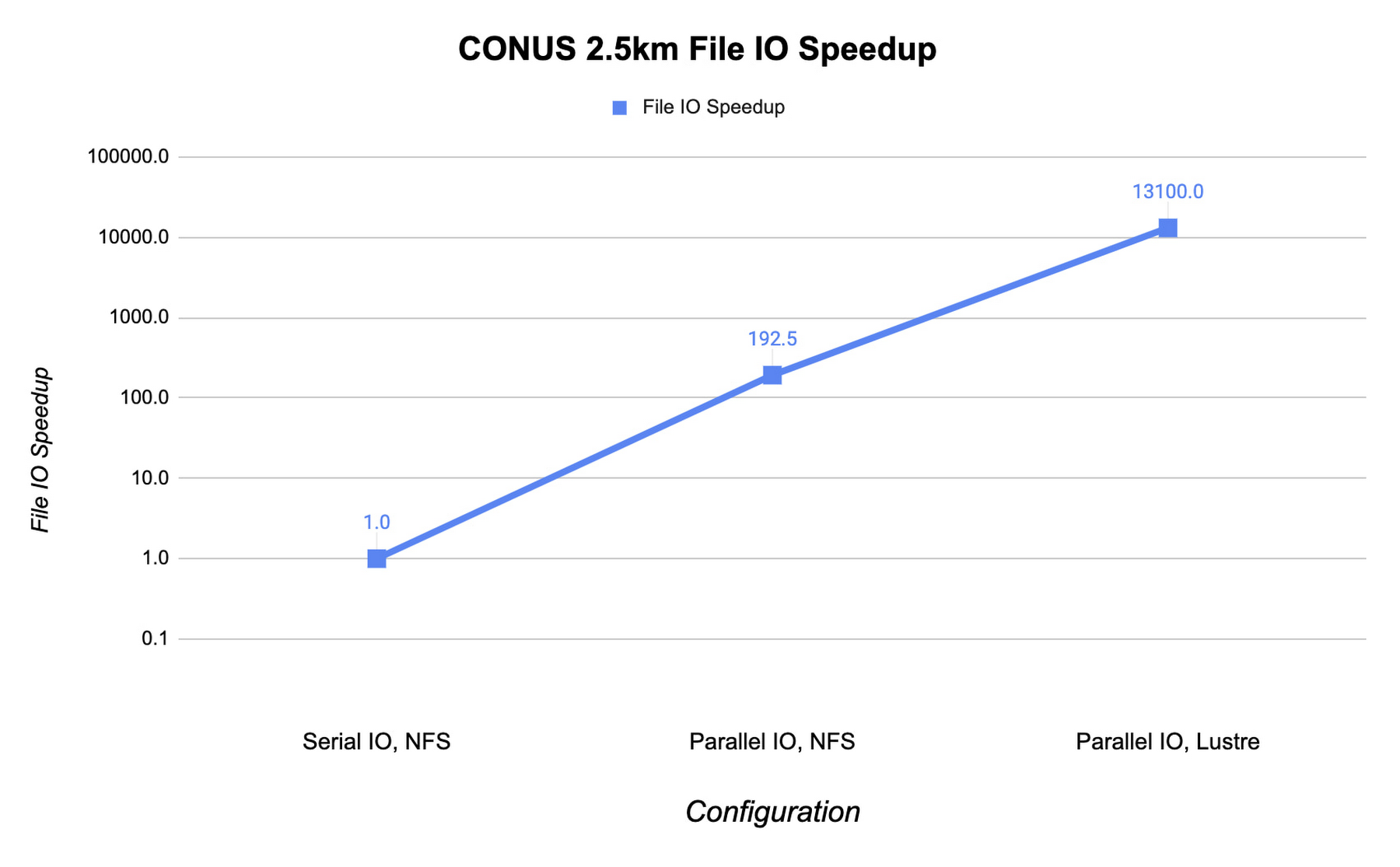
Below, we show the speedup in file IO activities relative to serial IO on an NFS file system. For this example, we are running the CONUS 2.5km benchmark on c2-standard-60 instances with 960 MPI ranks. By changing WRF’s file IO strategy to parallel IO, we accelerate file IO time by a factor of 60. 

We further speed up IO and reduce simulation costs by using a Lustre parallel file system deployed from open-source Lustre Terraform infrastructure-as-code from Fluid Numerics. Lustre is also available with support from DDN’s EXAScaler solution in the Google Cloud Marketplace. In this case, we use four n2-standard-16 instances for the Lustre Object Storage Server (OSS) instances, each with 3TB of Local SSD. The Lustre Metadata Server (MDS) is an n2-standard-16 instance with a 1TB PD-SSD disk. After mounting the Lustre file system to the cluster, we set the Lustre stripe count to 4 so that file IO can be distributed across the four OSS instances. By switching to the Lustre file system for IO, we speed up file IO by an additional factor of 193, which is orders of magnitude faster than a single NFS server with serial IO.

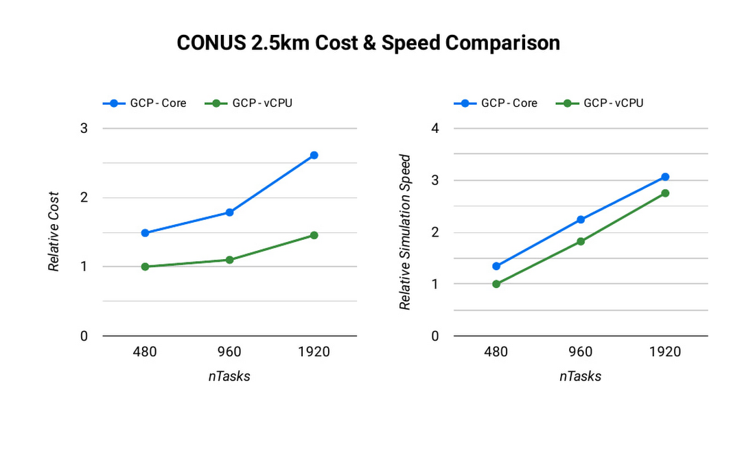
Adding compute resources and increasing the number of MPI ranks reduces the simulation run time. Ideally, with perfect linear scaling, doubling the number of MPI ranks would cut the simulation time in half. However, adding MPI ranks also increases communication overhead, which can increase the cost per simulation. The communication overhead is due to the increased amount of communication necessitated by splitting the problem more finely across more machines. 

To assess the scalability of WRF for the CONUS 2.5km benchmark, we can execute a series of model forecasts where we successively double the number of MPI ranks. Below, we show two- hour forecasts on the c2-standard-60 instances with the Lustre file system, varying the number of MPI ranks from 480 to 1920. In all of these runs, MPI ranks are bound to vCPUs so that the number of vCPUs dedicated to each simulation increases with the increase in MPI ranks. While many HPC workloads run best with simultaneous multithreading (SMT) disabled, we find the best performance for CONUS 2.5km with SMT enabled. Thus, the number of MPI ranks in our runs equals the total number of vCPUs.

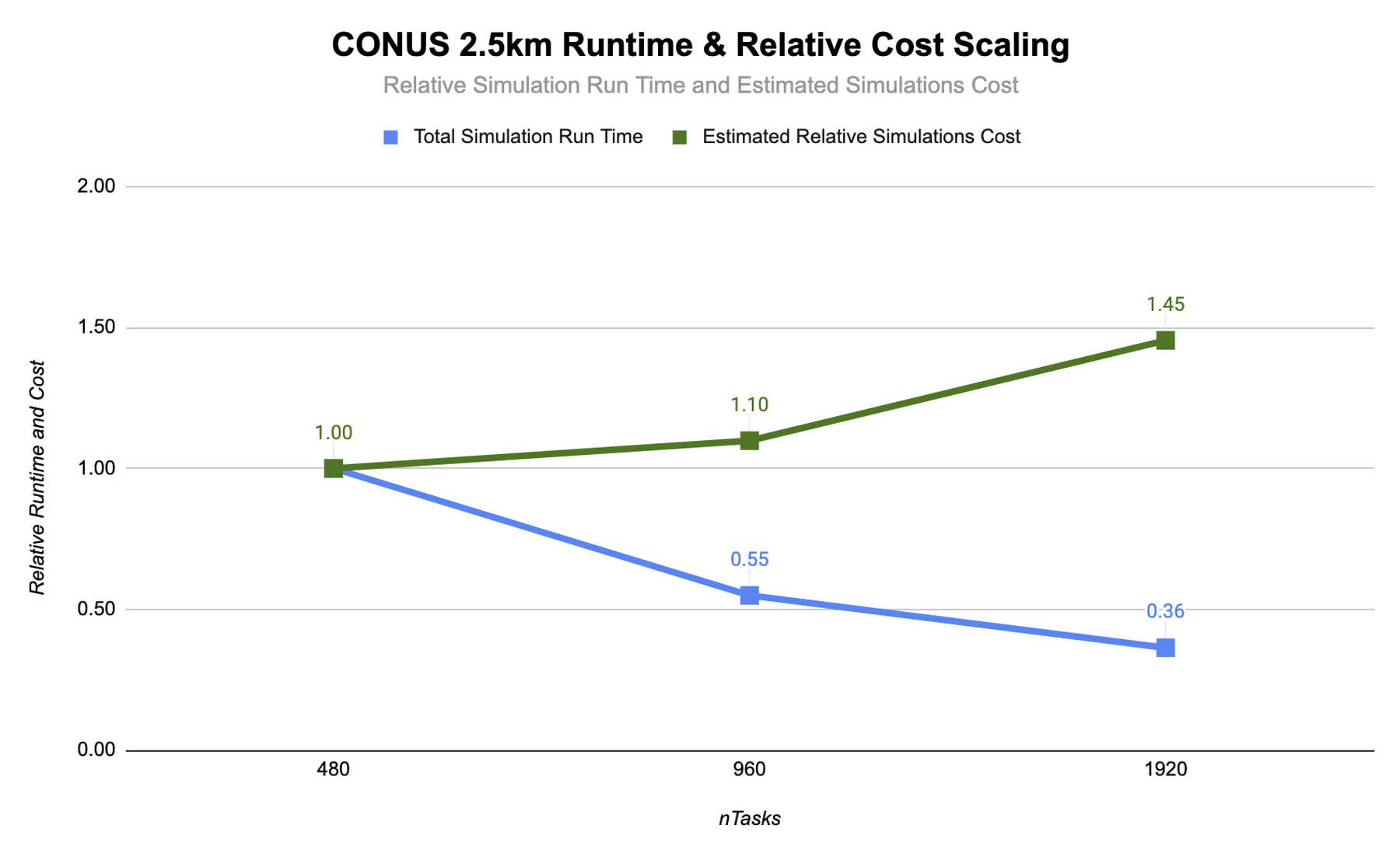
As you can see, the CONUS 2.5km Runtime & Cost Scaling figure shows that the run time (blue bars) decreases as the number of MPI ranks and the amount of compute resources increases, at least up to 1920 ranks. When transitioning from 480 to 960 MPI ranks, the run time drops, yielding a speedup of about 1.8x. Doubling again to 1920 MPI ranks, though, we obtained an additional speedup of just 1.5x. This declining trend in the speedup with increasing MPI ranks is a signature of MPI overhead, which increases with more MPI ranks.

Determining your best fit

Most tightly-coupled MPI applications such as WRF exhibit this kind of scaling behavior, where scaling efficiency decreases with increasing MPI ranks. This makes assessing cost-scaling alongside performance-scaling critical when considering Total Cost of Ownership (TCO). Thankfully, per-second billing on Google Cloud makes this kind of analysis a little bit easier. As shown above, a second doubling of the count from 960 cores to 1920 cores can provide an additional 1.5x speedup, but at a 32% higher cost. In some circumstances, this faster turnaround may be needed and worth the extra cost. 

If you want to get started with WRF quickly and experiment with the CONUS 2.5km benchmark, we’ve encapsulated this deployment in Terraform scripts and prepared an accompanying codelab.

You can learn more about Google Cloud’s high performance computing offerings at https://cloud.google.com/hpc, and you can find out more about Google’s partner Fluid Numerics at https://www.fluidnumerics.com.