Google Cloud

Using Google Cloud Machine Learning to predict clicks at scale

February 21, 2017

Andreas Sterbenz

Software Engineer

Google Cloud Machine Learning and TensorFlow are excellent tools for solving perception problems such as image classification. They work equally well on more traditional machine-learning problems such as click prediction for large-scale advertising and recommendation scenarios. To demonstrate this capability, in this post we'll train a model to predict display ad clicks on Criteo Labs clicks logs. These logs are over 1TB in size and contain feature values and click feedback from millions of display ads. We show how to train several models using different machine-learning techniques to predict the clickthrough rate.

The code for this example can be found here. Before following along below, be sure to set up your project and environment first. You should also make sure you have sufficient resource quota to process this large amount of data, or run on a smaller dataset as described in the example.

Preprocessing the data

The source data is provided as a set of text files by Criteo Labs. Each line in these files represents one training example as tab-separated-values (TSV) with a mix of numerical and categorical (string valued) features plus a label column indicating if the ad was clicked. We'll use Google Cloud Dataflow-based preprocessing to convert the 4 billion instances into Tensorflow Example format. As part of this process, we'll also build a vocabulary for the categorical features mapping them to integers, and split the input data into a training and evaluation sets. We use the first 23 days of data for the training set, and the 24th day for evaluation.

To start the Cloud Dataflow job, we run

This only takes around 60 minutes to run using autoscaling, which automatically chooses the appropriate number of machines to use. The output is written as compressed TFRecords files to Google Cloud Storage. We can inspect the list of files by running

Training a linear model

Next, we’ll train a linear classifier — that is, use a linear function to predict the value, which is a popular technique that scales well to large datasets. We use an optimization algorithm called Stochastic Dual Coordinate Ascent (SDCA) with a modification for multi replica training. It only needs a few passes over the data to converge and does not require the user to specify a learning rate.

For this baseline model, we’ll perform simple feature engineering. We use different types of feature columns to model the data. For the integer columns, we use a bucketized column, which groups ranges of input values into buckets:

Because the preprocessing step converted categorical columns to a vocabulary of integers, we use the sparse integerized column and pass the size of the vocabulary:

We train a model on Cloud Machine Learning by running the gcloud command. In addition to arguments used by gcloud itself, we also specify parameters that are used by our Python training module after the “--” characters:

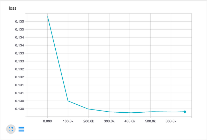
The configuration specifies using 60 worker machines and 29 parameter machine for training. With these settings, the model takes about 70 minutes to train and gives us an evaluation loss of 0.1293:

https://storage.googleapis.com/gweb-cloudblog-publish/images/criteo-1nhbm.max-800x800.PNG

Figure 1: Graph of the loss for the linear model

Adding crosses

We can improve on the model above by adding crosses, or combinations of two or more columns. This technique enables the algorithm to learn which non-linear combinations of features are relevant and improves the model’s predictive capability. We specify crosses using the crossed_column API:

For simplicity, we’ll use 1 million hash buckets for each crossed column. The combination of columns were determined empirically.Because we have 86 feature columns instead of 40, this model takes a bit longer to train — around 2.5 hours — but loss improves to 0.1272. While an improvement in loss of 1.5% may seem small, it can make a huge difference in advertising revenue or be the difference between first place and 15th place in machine-learning competitions.

Training a deep neural network

Linear models are quite powerful, but we can achieve better results by using a deep neural network (DNN). A neural network can also learn complex feature combinations automatically, removing the need to specify crosses.

In Tensorflow, switching between different types of models is easy. For the deep network we’ll use the same feature columns for the integer features. For the categorical columns, we’ll use an embedding column with the size of the embedding calculated based on the number of unique values in the column:

The only other change we make is to use a DNNClassifier from the learn package:

We again run gcloud to train the model. Neural networks can be arranged in many configurations. In this example, we use a simple stack of 11 fully connected layers with 1,062 neurons each.

This model is more complex and takes longer to run. Training for one epoch takes 26 hours, but loss improves to 0.1257. We can get even better results by training longer and reach a loss of 0.1250 after 78 hours. (Note that we used CPUs to train this model; for the sparse data in this problem, GPUs do not result in a large improvement.)

Comparing the results

The table below compares the different modeling techniques and the resulting training time and loss. We see the linear model is more computationally efficient and gives us a good loss quickly. But for this particular data set, the deep network produces a better result given enough time.

Modeling technique	Training time	Loss	AUC
Linear model	70 minutes	0.1293	0.7721
Linear model with crosses	142 minutes	0.1272	0.7841
Deep neural network, 1 epoch	26 hours	0.1257	0.7963
Deep neural network, 3 epochs	78 hours	0.1250	0.8002

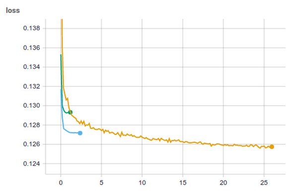
https://storage.googleapis.com/gweb-cloudblog-publish/images/criteo-25ce2.max-600x600.PNG

Figure 2: Graph of loss for the different models vs training time in hours.

Next steps

As you can see from this example, Cloud Machine Learning and Tensorflow make it easy to train models on very large amounts of data, and to seamlessly switch between different types of models with different tradeoffs for training time and loss.

If you have any feedback about the design or documentation of this example or have other issues, please report it on GitHub; pull request and contributions are also welcome. We're always working to improve and simplify our products, so stay tuned for new improvements in the near future!
See also: