Transform publicly available BigQuery data and Stackdriver logs into graph databases with Neo4j

The Google Cloud Partner Engineering team is excited to announce the availability of Neo4j Enterprise VM solution and Test Drive on Google Cloud Launcher.

Neo4j is very helpful whether your use case is better understanding NCAA Mascots or analyzing your GCP security posture with Stackdriver logs.  All of these use cases call for a high-performance graph database. Graph databases emphasize the importance of the relationship between data, and stores the connections as first-class citizens. Accessing nodes and relationships in a graph database makes for an efficient, constant-time operation and allows you to quickly traverse millions of connections quickly and efficiently.

In today’s blog post, we will give a light introduction to working with Neo4j’s query language, Cypher, as well as demonstrate how to get started with Neo4j on Google Cloud. You will learn how to quickly turn your Google BigQuery data or your Google Cloud logs into a graph data model, which you can use to reveal insights by connecting data points.

Let’s take Neo4j for a test drive.

Neo4j with NCAA BigQuery public datasets

Once you have either created or signed into your Orbitera account, you can deploy the Neo4j Enterprise test drive.

Exporting the NCAA BigQuery data

While we wait for our Neo4j graph to deploy, we can log into BigQuery and start to prepare a dataset for consumption by Neo4j.

1. Click here for the BigQuery Public Dataset page. (More background information can be found here.)
2. From this screen, click on the blue arrow of the mascots table, then click “export table”.

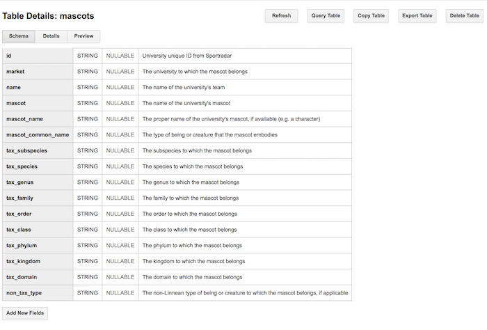
This will let you quickly and efficiently export the data associated with NCAA mascots into Google Cloud Storage as a CSV file.

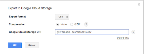
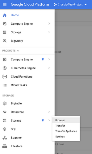
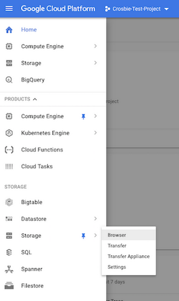
Find the Cloud Storage browser under Storage>Browser

Find the file you exported from BigQuery; ours is called mascots.csv. Since this is already a public dataset and does not contain sensitive data, the easiest way to give Neo4j access to this file is simply to share it publicly.

​

Click the checkbox under “Share publicly”

Connecting BigQuery data to the Neo4j test drive

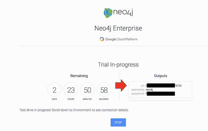
Now that our mascots data is accessible publicly, let’s return to our Neo4j test drive and on the trial status page, find the URL (url), username, and password.

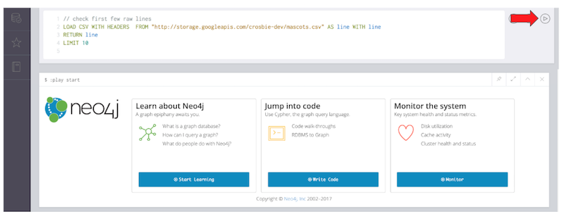
Once you are in the test drive browser check to make sure you can import the CSV mascots data: put the following code into the box at top, then press the play button on the right hand side.

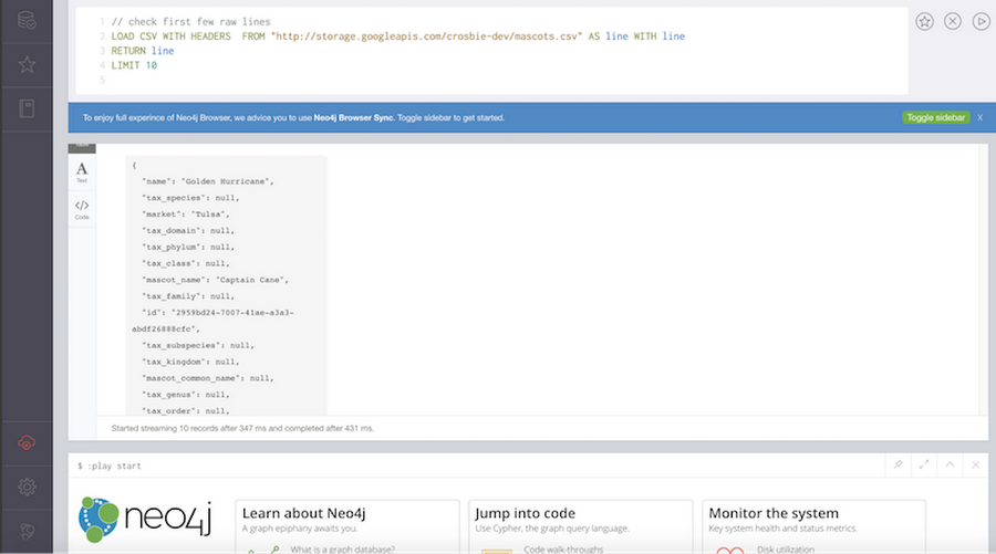
This query should return ten mascot results as text, as shown below.

Connecting BigQuery data to the Neo4j test drive

As an example of how to turn our mascots data into a very simple graph, simply run the below code in the Cypher block. This loads the data from your public Cloud Storage bucket and sets up some simple relationships in a graph data structure.

For each unique conceptual identity, we create a node. Each node will be given a label of either mascot, market, or the mascot’s taxonomic rank. A very basic relationship is also maintained between all of these elements with a relationship of either “location in” to associate the mascot and a market or an “is” relationship to indicate if the mascot is a certain biological classification. By using MERGE in Cypher, only one node is created for each unique value of things such as kingdoms, or phylums. In this way, we ensure that all the mascots of the same kingdom are linked to the same node.  For a deeper discussion on Neo4j data modeling, see the developer guide.

When the query loading step is finished, you should see a return value of 274, the total number of records in the input file, which lets you know the query was successful.

One of the best ways to improve Neo4j graph performance is to make sure that each node has as index, which can be done with the following code. Each index statement must run in separate code blocks.

Exploring the NCAA mascot graph with Cypher

To see what our NCAA mascot graph looks like, run the below Cypher query. This query builds a graph based on when a mascot node contains the name “Buckeye”.

This query should return a graph similar to the following image.

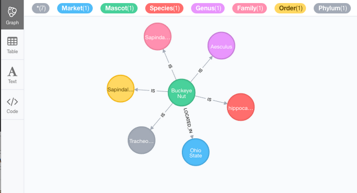
We can quickly see a mascot (node) containing Buckeye Nut {label} is located in [relationship] of the market(node) of Ohio State. {label}

You can also see that each of the taxonomic ranks for a Buckeye also have an “IS” relationship. We could extend the complexity of this graph by creating relationships that maintain the hierarchy of the taxonomic rank but since we are just introducing the concept of converting BigQuery data to a graph, we will continue with this simple graph structure.

Tigers and eagles and bulldogs, oh my!

While the true power of Cypher is that it allows us to explore relationships within the data, it is also useful in providing the same type of aggregations on the data that SQL gives us. Use the below query to find the three most popular types of mascots in the NCAA. The query result should be a visualization that lets you quickly identify tigers, eagles, and bulldogs as the most common mascots in the NCAA. The visualization also lets us identify the various markets that are home to these mascots.

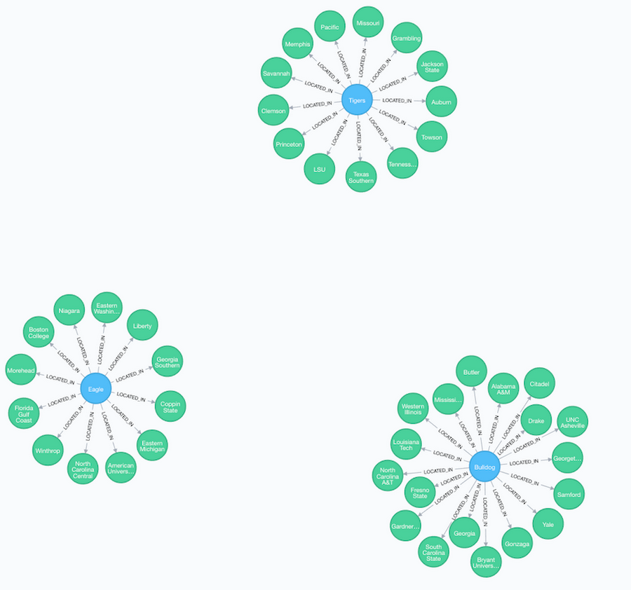
Neo4j’s Browser displays the result in this graphical way because the return type of the query contained nodes and edges. If we wanted a more traditional tabular style result, we can modify the query to request only certain attributes, such as:

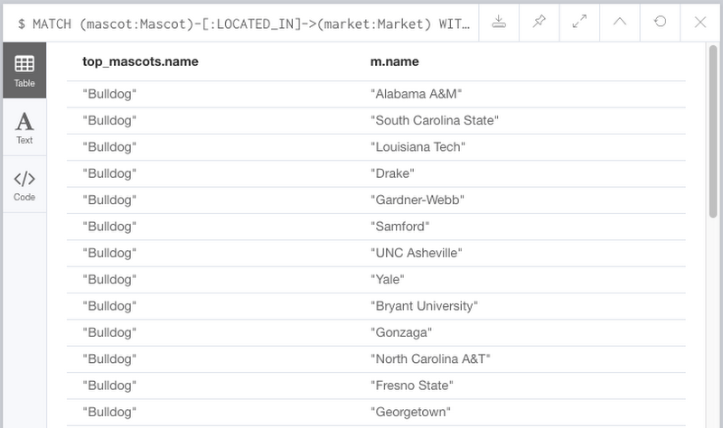
We can now modify this query to find the three most popular mascots that are human as opposed to an animal.

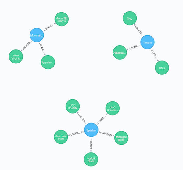
What do a Buckeye Nut and an Orange have in common?

Because Neo4j is a graph database, we can use the taxonomy structure in the data to find the shortest paths between nodes, to give a sense of how biologically similar two different kinds of things are, or at least what attributes they share. All we need is to match two different nodes in the graph, and then ask for all of the shortest paths connecting them, like so:

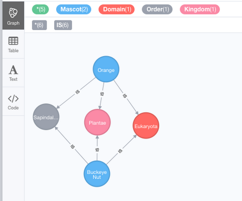
Here, the graph patterns are showing us that a buckeye nut and an orange share several classifications; they’re all plants, all Eukaryotes, and all in the Sapindales order, which are flowering plants.

Completing our test drive

At this point, we’ve seen how easy it is to get started using Neo4j in a contained environment, how we can quickly convert a BigQuery public dataset into a graph structure, and how we can interrogate the graph using aggregation capabilities.
Now the real fun of using a graph data starts! In Cypher, run:

:play start

This command will launch a card of Neo4j tutorials. Following those guides will let you understand the real power of having your data structured as a graph.
In our next section, we will move from test driving Neo4j with our public datasets into a private implementation of Neo4j that we can use to better understand our GCP security posture.

Using Neo4j to understand Google Cloud monitoring data

Cloud infrastructure greatly increases the security posture of most enterprises, but it can also increase the sophistication of the configuration management databases (CMDB). We need tools  to understand the varied and ephemeral relationships of IT assets in the cloud. A graph database such as Neo4j can enable you to better understand your full cloud architecture by providing the ability to easily connect data relationships all the way from the Kubernetes microservices that collect the data to the rows in a BigQuery analysis where the data ends up in. For more on how Neo4j can help with similar use cases to this one, see the Manage and Monitor Your Complex Networks with Real-Time Insight white paper.

In this section, we will use Stackdriver Logging to collect BigQuery logs and then export them into a Neo4j graph. For easy understanding, this graph will be limited to small subset of BigQuery logs but the real value of the relationships in Stackdriver data is once you expand your graph with logs across VMs, Kubernetes, various Google Cloud services and even AWS.

Neo4j causal clustering

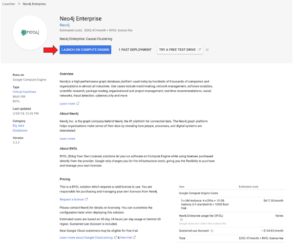
Unlike the NCAA public data, our stackdriver logs will most likely contain a lot of sensitive data we would not want to put on a test drive or expose publicly. The easiest way to obtain a fault tolerant Neo4j database in our private Google Cloud project is by using GCP Launcher’s Neo4j Enterprise deployment.
Simply click this link and then click the “Launch on Compute Engine” button as shown below.

Once you obtain a license from Neo4j and populate the configuration on the next page, a Neo4j cluster is deployed into your project that provides:

• A fault-tolerant platform for transaction processing that remains available even if there is a VM failure
• Scale through read replicas
• Causal consistency, meaning a client application is guaranteed to read at least its own writes.

Exporting Stackdriver metrics to the Neo4j virtual machine

From within the Google Cloud Platform console, you can go to Stackdriver>Logging-Exports as show below to create an export of your Stackdriver logs. In a production environment, you might set up an export to send logs to a variety of services. The example shown is similar to the export technique used for the NCAA mascot data above. Logs are collected in Stackdriver, exported to BigQuery, then BigQuery is used to export a CSV into Cloud Storage. In this particular graph, we limited our output to the results of the following BigQuery standard SQL query:

You can also export the logs directly from Stackdriver into Google Cloud Storage, creating JSON files. To import those JSON files, usually you’d install the APOC server extension for neo4j, but to keep things simple we’ll just use CSV for this example.

Note An important distinction between my process for importing public data from Cloud Storage, as compared with importing log data from Cloud Storage, is that I do not make the log data publicly available. I copy the log files to a local file on the Neo4j VM running in my account. I do so via SSH connection to the instance, then I run the below command in a directory to which the Neo4j processing has access.

The Neo4j Launcher deployment already provides the necessary read scopes for Google Cloud Storage to make this possible. However, you may still need to provide the service account of the Neo4j Compute Engine instance permissions to your bucket.

Stackdriver as a graph

Let’s start off by converting this sample Stackdriver data into a graph:

Even with this small subset of Stackdriver data, we can begin to see the value of having a Neo4j graph and Stackdriver working in tandem. Let’s take an example where we have used the Stackdriver Alerting feature’s built in condition to detect an increase in logging byte count.

When you create the below condition in Stackdriver, you can group the condition by both severity and the specific GCP project where the increase in logs is occurring.

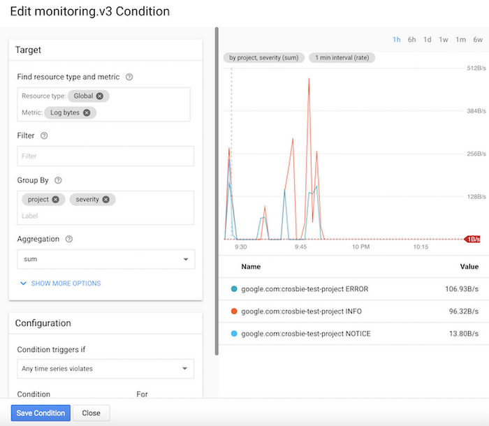
Once this configuration is setup, we can have Stackdriver alert me when a threshold of my choosing is crossed:

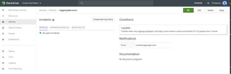
This threshold setting will help notify us that a particular GCP project is experiencing an increase in error logs. However with just this alert, we may need additional information to help diagnose the problem.This is where having your Stackdriver logs in Neo4j can help. Although this alert tells us to look in a particular project for a increase in error logs, having the graph available makes it possible to quickly identify the root cause by looking at the relationships contained in those GCP project logs.

Running the above query will give us the ERROR logs in a particular project but will also show the resource relationships associated with those logs, as well as any other type of node that has a relationship with our logs. The below image is the output result of the query:

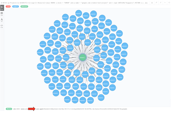
This single query makes it apparent that the error logs (nodes in blue) in the project are all attributed not only to a single resource of “BigQuery” but also to a specific node which contains the same method type and HTTP user agent header. This single node tells us that BigQuery query jobs coming from the Chrome browser are responsible for the increase in errors in the project and gives us a good place to start investigating the issue.

To learn more about using Neo4j to model your network and IT infrastructure run the command:

:play https://guides.neo4j.com/gcloud-testdrive/network-management.html

Conclusion

To get started for free, check out the Test Drive on Google Cloud Launcher.