Google Cloud Platform for Data Scientists: Using R with Google Cloud SQL for MySQL

By connecting R to Cloud SQL, you can take advantage of all R features on top of a scalable, fully-managed MySQL service.

Many developers working with relational data store aspects of business logic, customer metrics and other business data in a MySQL database. When data scientists or analysts outside the software development team analyze the data for insights, they may well choose the popular R programming language for creating statistical summaries and publication-quality visualizations of the data. But first, to get to the data from the shared data store, those users will need to connect to MySQL from R.

Google Cloud SQL is a relational database service in Google Cloud Platform (GCP) that's easy to maintain and access from a variety of programming languages and data platforms. Using Cloud SQL, developers who are familiar with PostgreSQL (public beta announced at Google Cloud NEXT '17) or MySQL can record, manipulate and migrate data without needing to manage their own hardware and can scale up technical infrastructure without time-consuming migrations.

Connecting R to Cloud SQL Second Generation is as easy as connecting to any MySQL database. The only difference is that you'll need to use the Cloud SQL Proxy for bridging the connection between the R client and Cloud SQL. That difference aside, you can access Cloud SQL from your R programs just as you would any other SQL database.

In this post—part of an open-ended series devoted to using GCP as a platform for doing data science at scale—I’ll take you through the following high-level steps:

1. Create a Cloud SQL Instance
2. Configure access to the instance
3. Add a user and verify everything is working
4. Query the data using R

Create a Cloud SQL Instance

• This tutorial assumes that you're using a Cloud SQL Second Generation instance.
• The instance value passed to commands is typically the instance connection name, which is in the properties page of each Cloud SQL instance, selected from the Cloud SQL instances page.

Configure access to the instance

If you haven't already, install a MySQL client on your machine. On Windows, you use the MySQL installer. On OSX, you can install the mysql package using Homebrew:

Install the Cloud SQL Proxy as described in the documentation. As an example, the following command will download the proxy for OSX and enable execute permissions:

Now that you have the requisite tools and a Cloud SQL instance, it's time to configure the root user password and look up the Instance Connection Name from the developer console.

• Configure the root user account as described in the Cloud SQL documentation.
• Select the Cloud SQL instance you created from the Cloud SQL instances page.
• After you select the Cloud SQL instance, find the Instance Connection Name from the properties listed at the bottom of the page. The connection name is necessary for connecting to your Cloud SQL instances.

Add a user and verify everything works

First, in a bash shell, use the cloud_sql_proxy command to connect to your instance:

If the command succeeds, you'll see the following message returned to your shell:

You now can connect to the Cloud SQL proxy using familiar MySQL tools. Connect to the MySQL proxy using the mysql commandline client:

From the mysql commandline client, add a user so that you don't need to connect as root:

Disconnect from the server and then flush the privileges table using mysqladmin:

Now you should be able to connect as the user using the mysql client:

Verify everything's working by creating an example database and a basic table for testing:

Insert some data into the new table:

If everything's working, go ahead and add a few more rows to the table, if you want.

3. Query the data using R

Load the library and create a helper function to return a connection to the Cloud SQL instance using the proxy that you started in the previous section:

Now, you can run commands and store the results in R variables—for example, the following R REPL code:

lists the tables in the database to which you connected. To query for data in the table we created in the previous step, do the following from R:

Now you can access the table rows in the data variable, for example, you can print the value column as:

Now you can manipulate and plot table data directly from the Cloud SQL instance in R.

Plotting data from sample databases

If it's not already running, start the Cloud SQL proxy from your shell using the cloud_sql_proxy command:

After you have downloaded the zip file, unzip it into a temporary folder, connect to the Cloud SQL proxy, and then import the sample table using the mysql client from your shell:

Now you can look at the world data from Cloud SQL from the mysql client:

After retrieving the table descriptions, open your R REPL and query for summary data about countries:

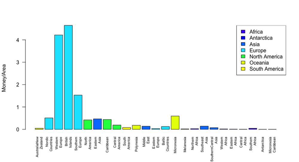
Now the world country data is ready for manipulation and plotting. Let's create a bar plot of Regional GNP Units (money) relative to land area using the following R code:

There are some interesting outliers in the data, such as British Islands and Western Europe.

As another example, let’s say you’re interested in the relationship between life expectancy and GNP per person. The following R REPL generates a plot that could lead to insights:

You can see there's a diminishing return in the increase of life expectancy relative to GNP around 5-thousandths of a GNP unit per person, that Antarctica doesn't have any living people and that African regions have lower life expectancy as well as lower GNP per person.

Next steps

Note that in production systems, you typically will want to be performing analytical operations outside of your master database. For this task, you could create a READ replica of your production database and then would use that replicant for long-running queries to avoid affecting the performance of your master database.

As you further improve your database management, you may want to programmatically perform these operations as demonstrated in the Cloud SQL sample code. If you're working with data that exceeds the limits of MySQL's scalability, you should check out Google BigQuery. (We’ll cover that subject in a future blog post.)

To dive deeper into using R with Cloud SQL:

• Check out the language reference for R on the CRAN site
• Explore Google Cloud SQL documentation