Google Cloud

Google Cloud Platform for data scientists: using Jupyter Notebooks with Apache Spark on Google Cloud

February 27, 2017

Reza Rokni

Senior Developer Advocate, Dataflow

James Malone

Product Manager, Google Cloud

Using the combination of Jupyter Notebooks and GCP gives you a familiar data science experience without the tedious infrastructure setup.

If you’re a data scientist, you probably prefer to spend your time exploring and analyzing your data, not thinking about sizing, installing and configuring your environment. If that sounds familiar, you’ll be happy to hear that using Jupyter Notebooks with the Google Cloud fully-managed big data stack gives you the notebook experience you know and love without having to burn hours on the boring infrastructure pieces. To demonstrate, in this post (which is part of an open-ended series about doing data science on GCP), we’ll walk you through the process of:

Creating a Jupyter notebook environment on Google Cloud Dataproc, a fully-managed Apache Spark and Hadoop service
Using the notebook to explore and visualize the public “NYC Taxi & Limousine Trips” dataset in Google BigQuery, Google’s fully-managed, cloud-native data warehouse service
Analyzing that data for a bit of a "hello world" type fun with Spark

Note that Google Cloud Datalab, a data exploration/analysis/visualization tool based on Jupyter, is another “no-ops” option for BigQuery, Google Compute Engine and Google Cloud Storage users. In this post, however, we’ll focus on using notebooks with Spark, which is more conveniently achieved by deploying Jupyter on Cloud Dataproc, as described here.

Prerequisites

Familiarity with Jupyter notebooks
A pre-existing GCP project (free trial)
An installed and authenticated gcloud command-line tool
Estimate the costs for running this lab based on Cloud pricing

Step 1: Get a Cloud Dataproc cluster up and running

In this step, you'll create a Cloud Dataproc cluster named "datascience" with Jupyter notebooks initialized and running using the command line. (Note: Please do not use Cloud Shell as you will not be able to create a socket connection from it in Step 2.)

The simplest approach is to use all default settings for your cluster. Jupyter will run on port 8123 of your master node. If you don't have defaults set, you'll be prompted at this stage to enter a zone for the cluster. As you'll be connecting to the UI on the cluster, choose zones in a region close to you.

(If you prefer using a graphical user interface, then the same action can be taken by following these instructions.)

Once completed, your Cloud Dataproc cluster is up and running and ready for a connection.

For the next step, you'll need to know the hostname of your Cloud Dataproc master machine as well as the zone in which your instance was created. To determine that zone, run the following command in your terminal:

Output:

The cluster master-host-name is the name of your Cloud Dataproc cluster followed by an -m suffix. For example, if your cluster is named "my-cluster", the master-host-name would be "my-cluster-m".

Step 2: Connect to the Jupyter notebook

You'll use an ssh tunnel from your local machine to the server to connect to the notebook. Depending on your machine’s networking setup, this step can take a little while to get right, so before proceeding confirm that everything is working by accessing the YARN UI. From the browser that you launched when following the instructions in the cluster-web-interfaces cloud documentation, access the following URL.

http://datascience-m:8088/

Once you have the tunnel running, connect to the external IP of the notebook and port. The default port is 8123.

http://datascience-m:8123

https://storage.googleapis.com/gweb-cloudblog-publish/images/jupyter-2h3or.max-1000x1000.PNG

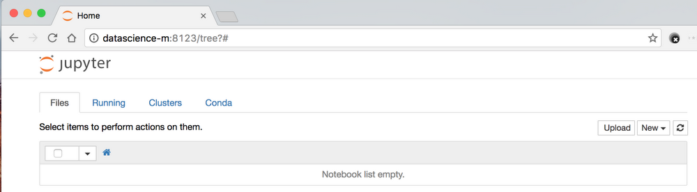
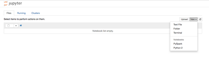
Step 3: Create a new notebook and add libraries Create a new PySpark notebook by clicking the new button on the Jupyter UI.

https://storage.googleapis.com/gweb-cloudblog-publish/images/jupyter-1z0fo.max-700x700.PNG

Everyone will have their own preferred selection of libraries, and adding new ones to the environment is simple. In this example, we'll ensure that pandas, google-api-python-client and seaborn are available.

In your notebook, run the following code cell:

(Note: The default Cloud Dataproc cluster configuration has been setup to work with one PySpark notebook kernel, so ensure you only have one notebook active at a time. Although you can change the configuration to be able to work with multiple running kernels, that process is beyond our scope here.)

Step 4: Run some queries and visualize results

In this step, you'll use the public NYC taxi dataset available in BigQuery to pull some data into a dataframe and visualize it. (Note: The pandas.io.gbq library is used in the examples below because the result set of the queries is small enough to be quickly transferred to the Cloud Dataproc node by paging through the resultset. If there's a need to pull a large dataset into Cloud Dataproc, however, the BigQuery Connector for Spark is a better choice.)

To import the required libraries, run the following in a cell.

To set up the project-id that you'll use, run the following in a cell.

Next, run a query to find the 50th, 75th and 90th quantiles against the nyc-tlc:yellow dataset. BigQuery will process 130GB of data containing 1,108,779,463 rows. The result set will be 24 rows of data that will be pulled into the notebook.

Run the following code in a cell.

Output

	pickup_hour	fiftieth	seventy_fifth	ninetieth
0	0	1	2	4
1	1	1	2	4
2	2	1	2	3
3	3	1	2	4
4	4	1	2	3

This next step will visualize the result set stored in trips. Run the following in a cell.

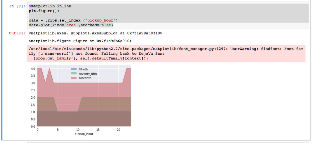
https://storage.googleapis.com/gweb-cloudblog-publish/images/jupyter-3rrzo.max-1000x1000.PNG

Step 5: Work with a Spark Dataframe and RDD

As described in Step 4, whereas the pandas.io.gbq library is great for pulling smaller results sets into the machine hosting the notebook, the BigQuery Connector for Spark is a better choice for larger ones. Although the example below uses the former for continuity purposes, in the real world, you would likely consider using the latter.

The query below works with the nyc-tlc:green dataset using trips from 2015; the predicate also further restricts the number of rows retrieved to just 1.5M. It should take approximately 2 mins to pull the rows into the notebook.

Output:

	pickup_datetime	passenger_count
0	2015-01-23 09:33:07	6
1	2015-01-11 19:06:34	1
2	2015-01-24 03:30:21	1
3	2015-01-08 04:18:58	1
4	2015-01-25 00:44:34	1

In the next step, a Spark DataFrame is created using sqlContext and some approximate quantiles are calculated with the error value moving from 1.0 down to 0.0.

Output:

In this next step, a RDD is created from the Spark DataFrame and a "hello world" mean is calculated.

Output:

Cleaning up

You can save your work by downloading the notebook and storing the file on your workstation. To delete the cluster (remember, ALL work will be deleted), run the following command on your workstation.