Easy distributed training with TensorFlow using tf.estimator.train_and_evaluate on Cloud ML Engine

TensorFlow’s version 1.4 release introduced the tf.estimator.train_and_evaluate function, which simplifies training, evaluation, and exporting of Estimator models. It abstracts away the details of distributed execution for training and evaluation, while also supporting consistent behavior across local/non-distributed and distributed configurations.

This means that with tf.estimator.train_and_evaluate you can run the same code both locally and distributed in the cloud, on different devices and using different cluster configurations, and get consistent results without making any code changes. When you’re done training (or at intermediate stages), the trained model is automatically exported in a form suitable for serving (e.g. for Cloud ML Engine online prediction or TensorFlow serving).

In this post, we’ll walk through how to use tf.estimator.train_and_evaluate with an Estimator model, and then show how easy it is to do distributed training of the model on Cloud ML Engine, moving between different cluster configurations with just a config tweak. The TensorFlow code itself supports distribution on any infrastructure—Google Cloud Engine, Google Container Engine, Google App Engine, etc.—when properly configured, but we will focus on Cloud ML Engine, which makes the experience seamless.

The primary steps necessary to do this are:

• Build your Estimator model.
• Define how data is fed into the model for both training and test datasets (often these definitions are essentially the same).
• Define training and eval specifications (TrainSpec and EvalSpec) to be passed to tf.estimator.train_and_evaluate. The EvalSpec can include information on how to export your trained model for prediction (serving), and we’ll look at how to do that as well.

The example also includes the use of Datasets to manage our input data. This API is part of TensorFlow 1.4 and is an easier and more performant way to create input pipelines to TensorFlow models; this is particularly important with large datasets and when using accelerators.

For our example, we’ll use the Census Income Data Set¹ hosted by the UC Irvine Machine Learning Repository. We have hosted the data on Google Cloud Storage in a slightly cleaned form. We’ll use this dataset to predict income category based on various information about a person.

This post omits some of the details of the example, so we’ve shared a Jupyter notebook to serve as a hands-on example. (The example in the notebook and its associated source code is a slightly modified version of this example).

Step 1: Create an Estimator

For this example, we’ll create an Estimator object using a pre-made subclass, DNNLinearCombinedClassifier, which implements a “wide and deep” model. Wide and deep models use a deep neural net (DNN) to learn high level abstractions about complex features or interactions between such features. These models then combine the outputs from the DNN with a linear regression performed on simpler features. This provides a balance between power and speed that is effective on many structured data problems.

See the accompanying notebook for how to define our Estimator, including specification of the expected input data format. The data is in CSV format, and looks like this:

We’ll use the last field, which indicates income bracket, as our label, meaning that this is the value we’ll predict based on the values of the other fields.

In the notebook, we define a build_estimator function, which takes as input config info, and returns a tf.estimator.DNNLinearCombinedClassifier object. We’ll call it like this:

Step 2: Define input functions using Datasets

We’ll use TensorFlow’s Dataset class to access our data. This API is a new way to create input pipelines to TensorFlow models. The Dataset API is much more performant than using feed_dict or the queue-based pipelines, and it’s cleaner and easier to use.

In this simple example, our datasets are too small for the use of the Dataset API to make a large difference, but with larger datasets it becomes much more important.

The input_fn definition is below. It uses a couple of helper functions that are defined in the accompanying notebook. One of these, parse_label_column, is used to convert the label strings (in our case, ‘ <=50K’ and ‘ >50K’) into one-hot encodings, which map categorical features into a format that works better with most ML classification models.

Then, we’ll use input_fn to define both the train_input and eval_input functions. We just need to pass input_fn the different source files to use for training versus evaluation. As we’ll see below, these two functions will be used to define a TrainSpec and EvalSpec used by train_and_evaluate.

Step 3: Define training and eval specifications

For our EvalSpec, we’ll instantiate it with something additional – a list of exporters, that specify how to export (save) the trained model so that it can be used for serving with respect to a particular data input format. Here we’ll just define one such exporter.

To specify our exporter, we must first define a serving input function. This is what determines the input format that the exporter will accept.

As we saw above, during training, an input_fn() ingests data and prepares it for use by the model.  At serving time, similarly, a serving_input_receiver_fn() accepts inference requests and prepares them for the model. This function has the following purposes:

• To add placeholders to the model graph that the serving system will feed with inference requests.
• To add any additional ops needed to convert data from the input format into the feature Tensors expected by the model.

A ServingInputReceiver is instantiated with two arguments — features and receiver_tensors. The features represent the inputs to our Estimator when it is being served for prediction. The receiver_tensors represent inputs to the server.

These two arguments will not necessarily always be the same — in some cases we may want to perform some transformation(s) before feeding the data to the model. Here’s one example of that, where the inputs to the server (csv-formatted rows) include a field to be removed.

However, in our case, the inputs to the server are the same as the features input to the model. Here’s what our serving input function looks like:

Then, we define an Exporter in terms of that serving input function. It will export the model in SavedModel format. We pass the EvalSpec constructor a list of exporters (here, just one).

Here, we're using the FinalExporter class.  This class performs a single export at the end of training. This is in contrast to LatestExporter, which does regular exports and retains the last N. (We’re just using one exporter here, but if you define multiple exporters, training will result in multiple saved models).

Step 4: Train your model using train_and_evaluate

tf.estimator.train_and_evaluate(estimator, train_spec, eval_spec)

This call will train the model and export the result in a format that is easy to use for prediction!

With train_and_evaluate, the training behavior will be consistent whether you run this function in a local/non-distributed context or in a distributed configuration.

The exported trained model can be served on many platforms. You may particularly want to consider ways to scalably serve your model, in order to handle many prediction requests at once—say if you’re using your model in an app you’re building, and you expect it to become popular. Cloud ML Engine online prediction and TensorFlow serving are two options for doing this.

In this post, we’ll look at using Cloud ML Engine Online Prediction. But first, let’s take a closer look at our exported model.

Examine the signature of the exported model

TensorFlow ships with a CLI that allows you to inspect the signature of exported SavedModel binary files—that is, the model’s inputs and outputs. This can be useful as a sanity check. We run it as follows, by passing it the path to directory containing the saved model, which will be called saved_model.pb. For our model, it will be found under $output_dir/export/census. This is because we passed the census name to our FinalExporter above. ($output_dir was specified when we constructed our Estimator).

The saved_model_cli command shows us this info (abbreviated for conciseness):

Based on our knowledge of DNNLinearCombinedClassifier and the input fields we defined, this looks as we expect. (Notice that the model generates multiple outputs).

Check local prediction with gcloud

We’ll use the example input in test.json to predict a person’s income bracket based on the features encoded in the test.json instance. Again, we point to the directory containing the saved model.

You can see how the input fields in test.json correspond to the inputs listed by the saved_model_cli command above, and how the prediction output probabilities correspond to the outputs listed by saved_model_cli. In this model, Class 0 indicates income <= 50k and Class 1 indicates income >50k.

Using Cloud ML Engine for easy distributed training and scalable online prediction

In this section, we’ll see how easy it is to use the same code—without any changes—to do distributed training on Cloud ML Engine, thanks to the Estimator class and train_and_evaluate. Then we’ll see how to use Cloud ML Engine Online Prediction to scalably serve the trained model.

One advantage of Cloud ML Engine is that there’s no lock-in. You could potentially train your TensorFlow model elsewhere, then deploy to Cloud ML Engine for serving (prediction); or alternately use Cloud ML Engine for distributed training and then serve elsewhere (e.g. with TensorFlow serving). Here, we’ll show how to use Cloud ML Engine for both stages.

To launch a training job on Cloud ML Engine, we can again use gcloud. We’ll need to package our code so that it can be deployed, and specify the Python file to run to start the training (--module-name).

The trainer module code is here. trainer.task is the entry point, and when that file is run, it calls tf.estimator.train_and_evaluate. (You can read more about how to package your code here).

If we want to, we could test (distributed) training via gcloud locally first, to make sure that we have everything packaged up correctly. See the accompanying notebook for details.

But here, we’ll jump right into using Cloud ML Engine to do cloud-based distributed training.

We’ll set the training job to use the SCALE_TIER_STANDARD_1 scale spec. This gives us one ‘master’ instance, plus four workers and three parameter servers.

The cool thing in the above snippet is that we don’t need to change our code at all to use this distributed config. Our use of the Estimator class in conjunction with the Cloud ML Engine scale specification makes the distributed training config transparent to us—it just works.

Further, we could swap in any of the other predefined scale tiers (say BASIC_GPU), or define our own custom cluster, again without any code changes. For example, we could alternatively configure our job to use a GPU cluster.

Once our training job is running, we can stream its logs to the terminal, and/or monitor it in the Cloud Console.

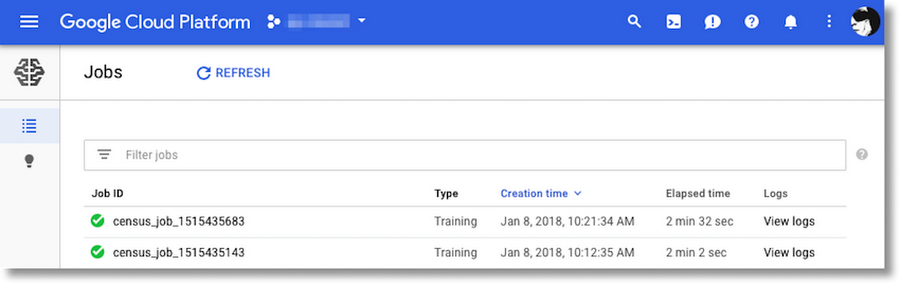
In the logs, you’ll see output from the multiple worker replicas and parameter servers that we utilized by specifying a SCALE_TIER_STANDARD_1 cluster. In the logs viewers, you can filter on the output of a particular node (e.g. a given worker) if you like.

Once your job is finished, you’ll find the exported model under the specified Google Cloud Storage directory, in addition to other data such as model checkpoints. That exported model has exactly the same signature as the locally-generated model we looked at above, and can be used in just the same ways.

Scalably serve your trained model with Cloud ML Engine online prediction

• Allocates some nodes the first time you request predictions, if there has been a long pause in requests.
• Scales the number of nodes in response to request traffic, adding nodes when traffic increases, and removing them when there are fewer requests.
• Keeps at least one node ready to handle requests even when there are none to handle. It then scales down to zero by default when your model version goes several minutes without a prediction request, but if you like, you can specify a minimum number of nodes to keep ready for a given model.

gcloud is great for testing your deployed model, and the command looks almost the same as it did for the local version of the model:

gcloud ml-engine predict --model census --version v1 --json-instances test.json

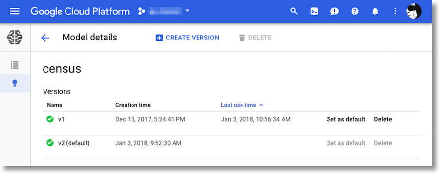
The Cloud Console makes it easy to inspect the different versions of a model, as well as set the default version: console.cloud.google.com/mlengine/models. You can list your model information using gcloud too.

Wrapping up

For more, see the accompanying notebook. The notebook includes examples of how to run your training job on a Cloud ML Engine GPU cluster and how to use Cloud ML Engine to do hyperparameter tuning.

¹The source of this dataset is from a third party. Google provides no representation, warranty, or other guarantees about the validity or any other aspects of this dataset.