Expanding your patent set with ML and BigQuery

Patents protect unique ideas and intellectual property. Patent landscaping is an analytical approach commonly used by corporations, patent offices, and academics to better understand the potential technical coverage of a large number of patents where manual review (i.e., actually reading the patents) is not feasible due to time or cost constraints. Luckily, patents contain rich information, including metadata (examiner-supplied classification codes, citations, dates, and information about the patent applicant), images, and thousands of words of descriptive text, which enable the use of more advanced methodological techniques to augment manual review.

Patent landscaping techniques have improved as machine learning models have increased practitioners’ ability to analyze all this data. Here on Google’s Global Patents Team, we’ve developed a new patent landscaping methodology that uses Python and BigQuery on Google Cloud to allow you to easily access patent data and generate automated landscapes.

There are some important concepts to know as you’re getting started with patent landscaping. Machine learning (ML) landscaping methods that use these sources of information generally fall into one of two categories:  

• Unsupervised: Given a portfolio of patents about which the user knows no prior information, then utilize an unsupervised algorithm to generate topic clusters to provide users a better high-level overview of what that portfolio contains.
• Supervised: Given a seed set of patents about which the user is confident covers a specific technology, then identify other patents among a given set that are likely to relate to the same technology. 

The focus of this post is on supervised patent landscaping, which tends to have more impact and be commonly used across industries, such as:

• Corporations that have highly curated seed sets of patents that they own and wish to identify patents with similar technical coverage owned by other entities. That may aid various strategic initiatives, including targeted acquisitions and cross-licensing discussions. 

• Patent offices that regularly perform statistical analyses of filing trends in emerging technologies (like AI) for which the existing classification codes are not sufficiently nuanced. 

• Academics who are interested in understanding how economic policy impacts patent filing trends in specific technology areas across industries. 

Whereas landscaping methods have historically relied on keyword searching and Boolean logic applied to the metadata, supervised landscaping methodologies are increasingly using advanced ML techniques to extract meaning from the actual full text of the patent, which contains far richer descriptive information than the metadata. Despite this recent progress, most supervised patent landscaping methodologies face at least one of these challenges:

• Lack of confidence scoring: Many approaches simply return a list of patents without indication of which are the most likely to actually be relevant to a specific technology space covered in the seed set. This means that a manual reviewer can’t prioritize the results for manual review, which is a common use of supervised landscapes. 

• Speed: Many approaches that use more advanced machine learning techniques are extremely slow, making them difficult to use on-demand. 

• Cost: Most existing tools are provided by for-profit companies that charge per analysis or as a recurring SaaS model, which is cost-prohibitive for many users. 

• Transparency: Most available approaches are proprietary, so the user cannot actually review the code or have full visibility into the methodologies and data inputs. 

• Lack of clustering: Many technology areas comprise multiple sub-categories that require a clustering routine to identify. Clustering the input set could formally group the sub-categories in a formulaic way that any downstream tasks could then make use of to more effectively rank and return results. Few (if any) existing approaches attempt to discern sub-categories within the seed set. 

The new patent landscaping methodology we’ve developed satisfies all of the common shortcomings listed above. This methodology uses Colab (Python) and GCP (BigQuery) to provide the following benefits:

• Fully transparent with all code and data publicly available, and provides confidence scoring of all results

• Clusters patent data to capture variance within the seed set

• Inexpensive, with sole costs incurring from GCP compute fee

• Fast, hundreds or thousands of patents can be used as input with results returned in a few minutes

Read on for a high-level overview of the methodology with code snippets. The complete code is found here, and can be reused and modified for your own ML and BigQuery projects. Finally, if you need an introduction to the Google Public Patents Datasets, a great overview is found here.

Getting started with the patent landscaping methodology 

1. Select a seed set and a patent representation
Generating a landscape first requires a seed set to be used as a starting point for the search. In order to produce a high-quality search, the input patents should themselves be closely related. More closely related seed sets tend to generate landscapes more tightly clustered around the same technical coverage, while a set of completely random patents will likely yield noisy and more uncertain results.

The input set could span a Cooperative Patent Code (CPC), a technology, an assignee, an inventor, etc., or a specific list of patents covering some known technological area. In this walkthrough a term (word) is used to find a seed set. In the Google Patents Public Datasets, there is a “top terms” field available for all patents in the “google_patents_research.publications” table. The field contains 10 of the most important terms used in a patent. The terms can be unigrams (such as “aeroelastic,” “genotyping,” or “engine”) or bi-grams (such as “electrical circuit,” “background noise,” or “thermal conductivity”).

With a seed set selected, you’ll next need a representation of a patent suitable to be passed through an algorithm. Rather than using the entire text of a patent or discrete features of a patent, it’s more consumable to use an embedding for each patent. Embeddings are a learned representation of a data input through some type of model, often with a neural network architecture. They reduce the dimensionality of an input set by mapping the most important features of the inputs to a vector of continuous numbers. A benefit of using embeddings is the ability to calculate distances between them, since several distance measures between vectors exist.

You can find a set of patent embeddings in BigQuery. The patent embeddings were built using a machine learning model that predicted a patent's CPC code from its text. Therefore, the learned embeddings are a vector of 64 continuous numbers intended to encode the information in a patent's text. Distances between the embeddings can then be calculated and used as a measure of similarity between two patents. 

In the following example query (performed in BigQuery), we’ve selected a random set of U.S. patents (and collected their embeddings) granted after Jan. 1, 2005, with a top term of "neural network."

2. Organize the seed set
With the input set determined and the embedding representations retrieved, you have a few options for determining similarity to the seed set of patents.

Let’s go through each of the options in more detail.

1. Calculating an overall embedding point—centroid, medoid, etc.— for the entire input set and performing similarity to that value. Under this method, one metric is calculated to represent the entire input set. That means that the input set of embeddings, which could contain information on hundreds or thousands of patents, ends up pared down to a single point. 

There are drawbacks to any methodology that is dependent on one point. If the value itself is not well-selected, all results from the search will be poor. Furthermore, even if the point is well-selected, the search depends on only that one embedding point, meaning all search results may represent the same area of a topic, technology, etc. By reducing the entire set of inputs to one point, you’ll lose significant information about the input set.

2. Seed set x N similarity, e.g., calculating similarity to all patents in the input set to all other patents. Doing it this way means you apply the vector distance metric used between each patent in the input set and all other patents in existence. This method presents a few issues: 

• Lack of tractability. Calculating similarity for (seed_set_size x all_patents) is an expensive solution in terms of time and compute. 

• Outliers in the input set are treated as equals to highly representative patents.

• Dense areas around a single point could be overrepresented in the results.

• Reusing the input points for similarity may fail to expand the input space.

3. Clustering the input set and performing similarity to a cluster. We recommend clustering as the preferred approach to this problem, as it will overcome many of the issues presented by the other two methods. Using clustering, information about the seed set will be condensed into multiple representative points, with no point being an exact replica of its input. With multiple representative points, you can capture various parts of the input technology, features, etc. 

3. Cluster the seed set
A couple of notes about the embeddings on BigQuery:

• The embeddings are a vector of 64 numbers, meaning that data is high-dimensional.

• As noted earlier, the embeddings were trained in a prediction task, not explicitly trained to capture the "distance" (difference) between patents.

Based on the embedding training, the clustering algorithm needs to be able to effectively handle clusters of varying density. Since the embeddings were not trained to separate patents evenly, there will be areas of the embedding space that are more or less dense than others, yet represent similar information between documents.

Furthermore, with high-dimensional data, distance measures can degrade rapidly. One possible approach to overcoming the dimensionality is to use a secondary metric to represent the notion of distance. Rather than using absolute distance values, it’s been shown that a ranking of data points from their distances (and removing the importance of the distance magnitudes) will produce more stable results with higher dimensional data. So our clustering algorithm should remove sole dependence on absolute distance.

It’s also important that a clustering method be able to detect outliers. When providing a large set of input patents, you can expect that not all documents in the set will be reduced to a clear sub-grouping. When the clustering algorithm is unable to group data in a space, it should be capable of ignoring those documents and spaces. 

Several clustering algorithms exist (hierarchical, clique-based, hdbscan, etc.) that have the properties we require, any of which can be applied to this problem in place of the algorithm used here. In this application, we used the shared nearest neighbor (SNN) clustering method to determine the patent grouping. 

SNN is a clustering method that evaluates the neighbors for each point in a dataset and compares the neighbors shared between points to find clusters. SNN is a useful clustering algorithm for determining clusters of varying density. It is good for high-dimensional data, since the explicit distance value is not used in its calculation; rather, it uses a ranking of neighborhood density. The complete clustering code is available in the GitHub repo.

For each cluster found, the SNN method determines a representative point for each cluster in order to perform a search against it. Two common approaches for representing geometric centers are centroids and medoids. The centroid simply takes the mean value from each of the 64 embedding dimensions. A medoid is the point in a cluster whose average dissimilarity to all objects in a cluster is minimized. In this walkthrough, we’re using the centroid method.

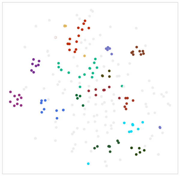
Below you’ll see a Python code snippet of the clustering application and calculations of some cluster characteristics, along with a visualization of the clustering results. The dimensions in the visualization were reduced using TSNE, and outliers in the input set have grayed out. The results of the clustering can be seen by the like colors forming a cluster of patents:

4. Perform a similarity search
Once the cluster groups and their centers have been determined, you’ll need a measure of similarity between vectors. Several measures exist, and you can implement any preferred measure. In this example, we used cosine distances to find the similarity between two vectors.

Using the cosine distance, the similarity between a cluster center is compared to all other patents using each of their embeddings. Distance values close to zero mean that the patent is very similar to the cluster point, whereas distances close to one are very far from the cluster point. You’ll see the resulting similarity calculations ordered for each cluster and get an upper bound number of assets.

Below you’ll see a Python code snippet that iterates through each cluster. For each cluster, a query is performed in BigQuery that calculates the cosine distance between the cluster center and all other patents, and returns the most similar results to that cluster, like this:

5. Apply confidence scoring
The previous step returns the most similar results to each cluster along with its cosine distance values. From here, the final step takes properties of the cluster and the distance measure from the similarity results to create a confidence level for each result. There are multiple ways to construct a confidence function, and each method may have benefits to certain datasets. 

In this walkthrough, we do the confidence scoring using a half squash function. The half squash function is formulated as follows:

The function takes as input the cosine distance value found between a patent and a cluster center (x). Furthermore, the function requires two parameters that affect how the distances of the results are fit onto the confidence scale:

1. A power variable, which defines the properties of the distribution showing the distance results—effectively the slope of the curve. In this version, a power of two is used.

2. A half value, which represents the midpoint of the curve returned and defines the saturation on either side of the curve. In this implementation, each cluster uses its own half value. The half value for each cluster is formulated as follows:
   (mean distance of input patents in cluster + 2 * standard deviation of input cluster distances)

The confidence scoring function effectively re-saturates the returned distance values to a scale between [0,1], with an exponentially decreasing value as the distance between a patent and the cluster center grows:

Results from this patent landscaping methodology
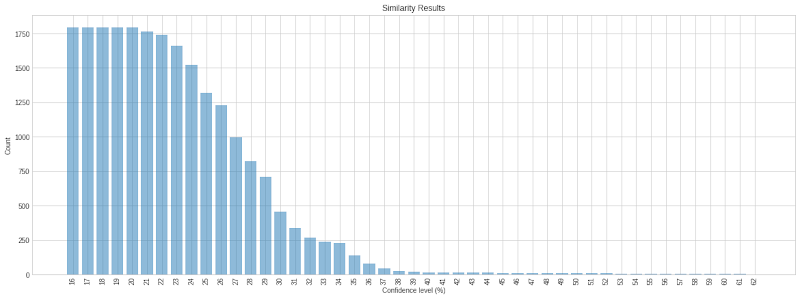
Applying the confidence function for all of the similarity search results yields a distribution of patents by confidence score. At the highest levels of confidence, fewer results will appear. As you move down the confidence distribution, the number of results increases exponentially.

Not all results returned are guaranteed to be high-quality; however, the higher the confidence level, the more likely a result is positive. Depending on the input set, the confidence levels will not necessarily begin at 99%. From the results above, using our “neural network” random patent set, the highest confidence results sit in the 60% to 70% range. From our own experimentation, the more tightly related the input set, the higher the confidence level in the results will be, since the clusters will be more compact.

This walkthrough provides one method for expanding a set of patents to generate a landscape. Several changes or improvements can be made to the cluster algorithm, distance calculations and confidence functions to suit any dataset. Explore the patents dataset for yourself, and try out GitHub for the patent set expansion code too.