Running TensorFlow inference workloads at scale with TensorRT 5 and NVIDIA T4 GPUs

Today, we announced that Google Compute Engine now offers machine types with NVIDIA T4 GPUs, to accelerate a variety of cloud workloads, including high-performance computing, deep learning training and inference, broader machine learning (ML) workloads, data analytics, and graphics rendering.

In addition to its GPU hardware, NVIDIA also offers tools to help developers make the best use of their infrastructure. NVIDIA TensorRT is a software inference platform for developing high-performance deep learning inference—the stage in the machine learning process where a trained model is used, typically in a runtime, live environment, to recognize, process, and classify results. The library includes a deep learning inference data type (quantization) optimizer, model conversion process, and runtime that delivers low latency and high throughput. TensorRT-based applications perform up to 40 times faster¹ than CPU-only platforms during inference. With TensorRT, you can optimize neural network models trained in most major frameworks, calibrate for lower precision with high accuracy, and finally, deploy to a variety of environments. These might include hyperscale data centers, embedded systems, or automotive product platforms.

In this blog post, we’ll show you how to run deep learning inference on large-scale workloads with NVIDIA TensorRT 5 running on Compute Engine VMs configured with our Cloud Deep Learning VM image and NVIDIA T4 GPUs.

Overview

This tutorial shows you how to set up a multi-zone cluster for running an inference workload on an autoscaling group that scales to meet changing GPU utilization demands, and covers the following steps:

• Preparing a model using a pre-trained graph (ResNet)

• Benchmarking the inference speed for a model with different optimization modes

• Converting a custom model to TensorRT format

• Setting up a multi-zone cluster that is:

• Built on Deep Learning VMs preinstalled with TensorFlow, TensorFlow serving, and TensorRT 5.

• Configured to auto-scale based on GPU utilization.

• Configured for load-balancing.

• Firewall enabled.  

• Running an inference workload in the multi-zone cluster.

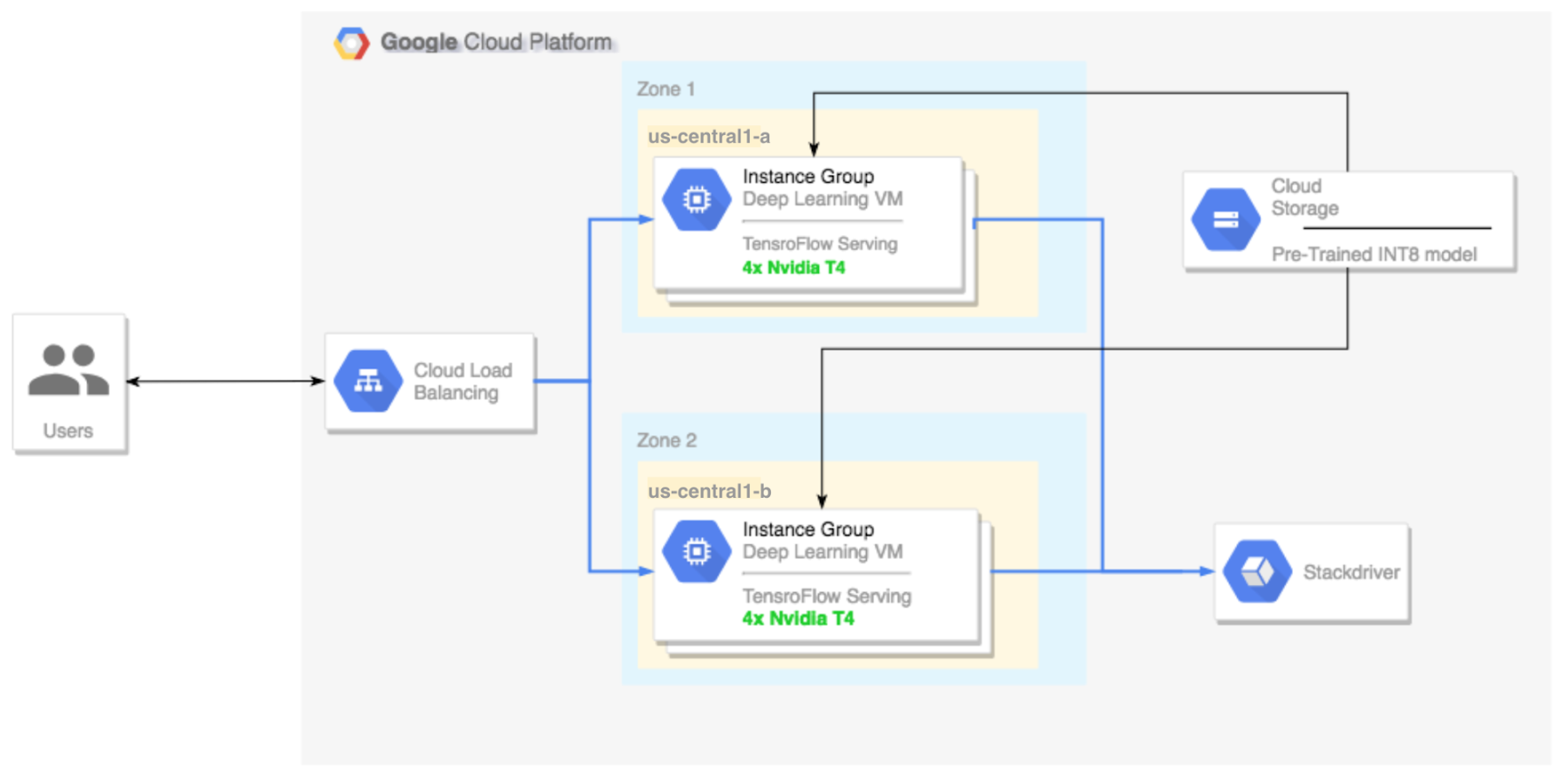
Here’s a high-level architectural perspective for this setup:

Preparing and optimizing the model with TensorRT

In this section, we will create a VM instance to run the model, and then download a model from the TensorFlow official models catalog.

Create a new Deep Learning Virtual Machine instance

Create the VM instance:

If command is successful you should see a message that looks like this:

Notes:

• You can create this instance in any available zone that supports T4 GPUs.

• A single GPU is enough to compare the different TensorRT optimization modes.

Download a ResNet model pre-trained graph

Verify model was downloaded correctly:

Save the location of your ResNet model in the $WORKDIR variable:

Benchmarking the model

Leveraging fast linear algebra libraries and hand tuned kernels, TensorRT can speed up inference workloads, but the most significant speed-up comes from the quantization process. Model quantization is the process by which you reduce the precision of weights for a model. For example, if the initial weight of a model is FP32, you have the option to reduce the precision to FP16 and INT8 with the goal of improving runtime performance. It’s important to pick the right balance between speed (precision of weights) and accuracy of a model. Luckily, TensorFlow includes functionality that does exactly this, measuring accuracy vs. speed, or other metrics such as throughput, latency, node conversion rates, and total training time. TensorRT supports two modes: TensorFlow+TensorRT and TensorRT native, in this example we use the first option.

Note: This test is limited to image recognition models at the moment, however it should not be too hard to implement a custom test based on this code.

Set up the ResNet model

To set up the model, run the following command:

This test requires a frozen graph from the ResNet model (the same one that we downloaded before), as well as arguments for the different quantization modes that we want to test.

The following command prepares the test for the execution:

Run the test

This command will take some time to finish.

Notes:

• $WORKDIR is the directory in which you downloaded the ResNet model.

• The --native arguments are the different available quantization modes you can test.

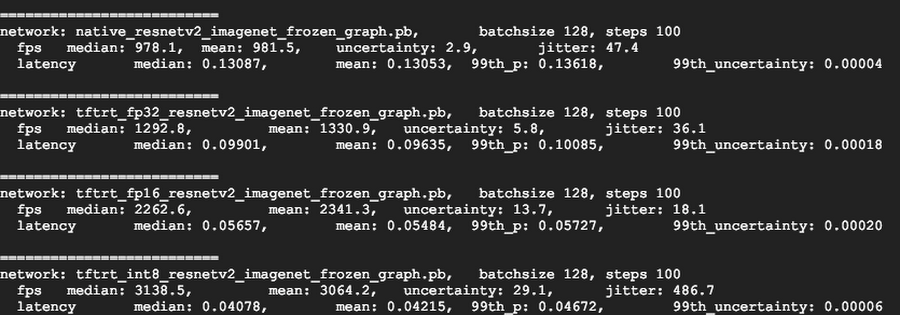
Review the results

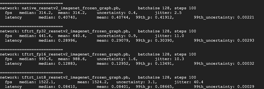
When the test completes, you will see a comparison of the inference results for each optimization mode.

To see the full results, run the following command:

V100

T4

P4

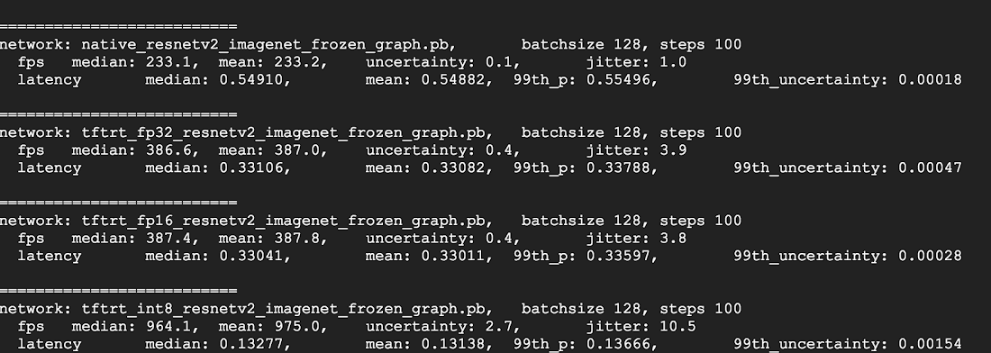
From the above results, you can see that FP32 and FP16 performance numbers are identical under predictions. This means that if you are content working with TensorRT, you can definitely start using FP16 right away. INT8, on the other hand, shows slightly worse accuracy and requires understanding the accuracy-versus-performance tradeoffs for your models.

In addition, you can observe that when you run the model with TensorRT 5:

• Using FP32 optimization improves throughput by 40% (440 vs 314). At the same time it decreases latency by ~30%, making it 0.28 ms instead of 0.40 ms.

• Using FP16 optimization rather than native TF graph increases the speed by 214%! (from 314 to 988 fps). At the same time latency decreased by 0.12 ms (almost 3x decrease!).

• Using INT8, the last result displayed above, we observed a speedup of 385% (from 314 to 1524) with the latency decreasing to 0.08 ms.

Notes:

• The above results do not include latency for image pre-processing nor HTTP requests latency. In production systems the inference’ speed may not be a bottleneck at all, and you will need to account for all the factors mentioned in order to measure your end to end inference’ speed.

Now, let’s pick a model, in this case, INT8.

Converting a custom model to TensorRT

Download and extract ResNet model

To convert a custom model to a TensorRT graph you will need a saved model. To download a saved INT8 ResNet model, run the following command:

SavedModels are generated to accept either tensor or JPG inputs, and with channels_first (NCHW) and channels_last (NHWC) convolutions. NCHW is generally better for GPUs, while NHWC is generally better for CPUs, in this case we are downloading a model that can handle JPG inputs.

Convert the model to a TensorRT graph with TFTools

Now we can convert this model to its corresponding TensorRT graph with a simple tool:

You now have an INT8 model in your $WORKDIR/resnet_v2_int8_NCHW/00001 directory.

To ensure that everything is set up properly, try running an inference test.

Upload the model to Cloud Storage

You’ll need to run this step so that the model can be served from the multi-zone cluster that we will set up in the next section. To upload the model, complete the following steps:

1. Archive the model.

2. Upload the archive.

If needed, you can obtain an INT8 precision variant of the frozen graph from Cloud Storage at this URL:

Setting up a multi-zone cluster

Create the cluster

Now that we have a model in Cloud Storage, let’s create a cluster.

Create an instance template

Notes:

• This instance template includes a startup script that is specified by the metadata parameter.

• The startup script runs during instance creation on every instance that uses this template, and performs the following steps:

• Installs NVIDIA drivers, NVIDIA drivers are installed on each new instance. Without NVIDIA drivers, inference will not work.

• Installs a monitoring agent that monitors GPU usage on the instance

• Downloads the model

• Starts the inference service

• The startup script runs tf_serve.py, which contains the inference logic. For this example, I have created a very small Python file based on the TFServe package.

• To view the startup script, see start_agent_and_inf_server.sh.

Create a managed instance group

You’ll need to set up a managed instance group, to allow you to run multiple instances in specific zones. The instances are created based on the instance template generated in the previous step.

Notes:

• INSTANCE_TEMPLATE_NAME is the name of the instance that you created in the previous step.

• You can create this instance in any available zone that supports T4 GPUs. Ensure that you have available GPU quotas in the zone.

• Creating the instance takes some time. You can watch the progress with the following command:

Once the managed instance group is created, you should see output that resembles the following:

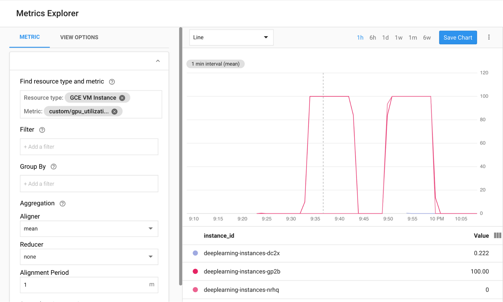
Confirm metrics in Stackdriver

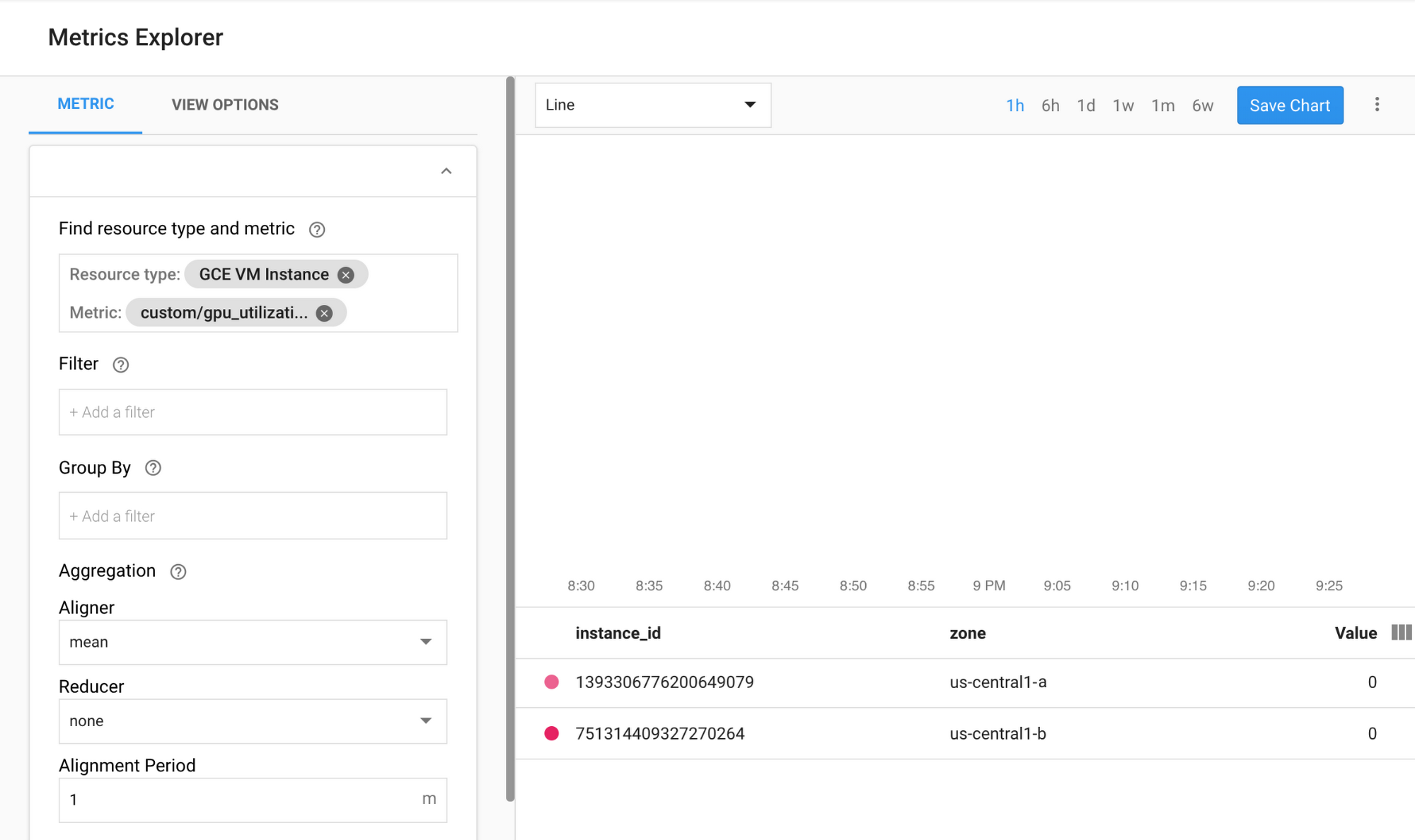
2. Search for gpu_utilization. StackDriver > Resources > Metrics Explorer

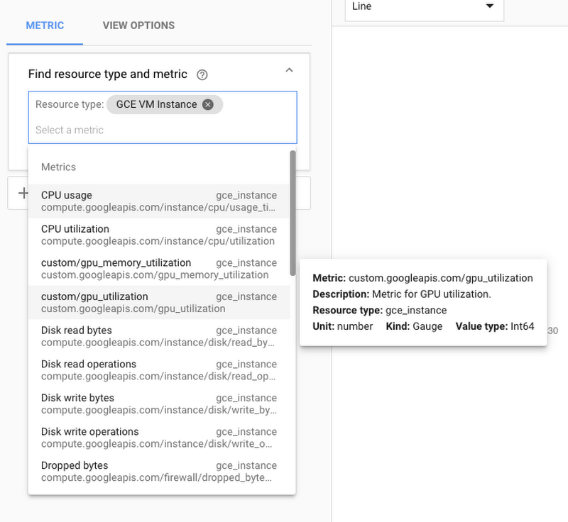
3. If data is coming in, you should see something like this:

Enable auto-scaling

Now, you’ll need to enable auto-scaling for your managed instance group.

Notes:

• The custom.googleapis.com/gpu_utilization is the full path to our metric.

• We are using level 85, this means that whenever GPU utilization reaches 85, the platform will create a new instance in our group.

Test auto-scaling

To test auto-scaling, perform the following steps:

1. SSH to the instances. See Connecting to Instances for more details.

Notes:

• During the make process, you may receive some warnings, ignore them.

• You can monitor the gpu usage information, with a refresh interval of 5 seconds:

3. You can observe the autoscaling in Stackdriver, one instance at a time.

4. Go to the Instance Groups page in the Google Cloud Console.

5. Click on the deeplearning-instance-group managed instance group.

6. Click on the Monitoring tab.

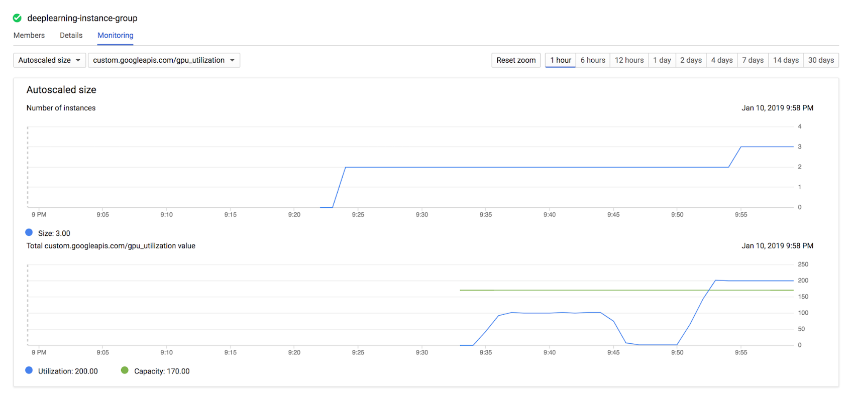
At this point your auto-scaling logic should be trying to spin as many instances as possible to reduce the load. And that is exactly what is happening:

At this point you can safely stop any loaded instances (due to the burn-in tool) and watch the cluster scale down.

Set up a load balancer

Let's revisit what we have so far:

• A trained model, optimized with TensorRT 5 (using INT8 quantization)

• A managed instance group. These instances have auto-scaling enable based on the GPU utilization

Now you can create a load balancer in front of the instances.

Create health checks

Health checks are used to determine if a particular host on our backend can serve the traffic.

Create inferences forwarder

Configure named-ports of the instance group so that LB can forward inference requests, sent via port 80, to the inference service that is served via port 8888.

Create a backend service

Create a backend service that has an instance group and health check.

First, create the health check:

Then, add the instance group to the new backend service:

Set up the forwarding URL

The load balancer needs to know which URL can be forwarded to the backend services.

Create the load balancer

Add an external IP address to the load balancer:

Find the allocated IP address:

Set up the forwarding rule that tells GCP to forward all requests from the public IP to the load balancer:

After creating the global forwarding rules, it can take several minutes for your configuration to propagate.

Enable the firewall

You need to enable a firewall on your project, or else it will be impossible to connect to your VM instances from the external internet. To enable a firewall for your instances, run the following command:

Running inference

You can use the following Python script to convert images to a format that can be uploaded to the server.

Finally, run the inference request:

That’s it!

Toward TensorFlow inference bliss

Running ML inference workloads with TensorFlow has come a long way. Together, the combination of NVIDIA T4 GPUs and its TensorRT framework make running inference workloads a relatively trivial task—and with T4 GPUs available on Google Cloud, you can spin them up and down on demand. If you have feedback on this post, please reach out to us here.

Acknowledgements: Viacheslav Kovalevskyi, Software Engineer, Gonzalo Gasca Meza, Developer Programs Engineer, Yaboo Oyabu, Machine Learning Specialist and Karthik Ramasamy, Software Engineer contributed to this post.

_{1. Inference benchmarks show ResNet training times to be 27x faster, and GNMT times to be 36x faster}