How to quickly solve machine learning forecasting problems using Pandas and BigQuery
Chris Rawles
ML Solutions Engineer
Ryan Gillard
Machine Learning Solutions Engineer
Time-series forecasting problems are ubiquitous throughout the business world. For example, you may want to predict the probability that some event will happen in the future or forecast how many units of a product you’ll sell over the next six months. Forecasting like this can be posed as a supervised machine learning problem.
Like many machine learning problems, the most time-consuming part of forecasting can be setting up the problem, constructing the input, and feature engineering. Once you have created the features and labels that come out of this process, you are ready to train your model.
A common approach to creating features and labels is to use a sliding window where the features are historical entries and the label(s) represent entries in the future. As any data-scientist that works with time-series knows, this sliding window approach can be tricky to get right.
Below is a good workflow for tackling forecasting problems:
1. Create features and labels on a subsample of data using Pandas and train an initial model locally
2. Create features and labels on the full dataset using BigQuery
3. Utilize BigQuery ML to build a scalable machine learning model
4. (Advanced) Build a forecasting model using Recurrent Neural Networks in Keras and TensorFlow
In the rest of this blog, we’ll use an example to provide more detail into how to build a forecasting model using the above workflow. (The code is available on AI Hub)
First, train locally
Machine learning is all about running experiments. The faster you can run experiments, the more quickly you can get feedback, and thus the faster you can get to a Minimum Viable Model (MVM). It’s beneficial, then, to first work on a subsample of your dataset and train locally before scaling out your model using the entire dataset.
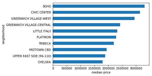
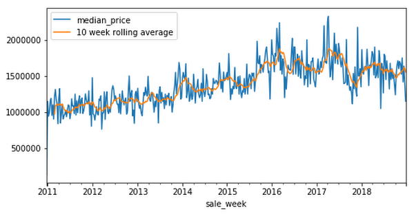
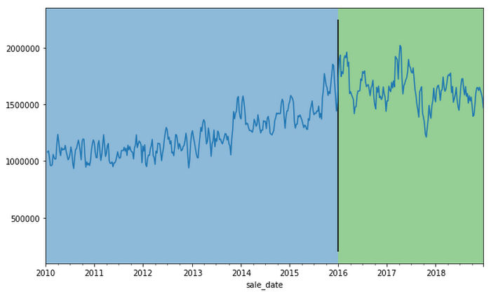
Let’s build a model to forecast the median housing price week-by-week for New York City. We spun up a Deep Learning VM on Cloud AI Platform and loaded our data from nyc.gov into BigQuery. Our dataset goes back to 2003, but for now let’s just use prices beginning 2011.
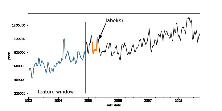
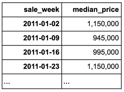
Since our goal is to forecast future prices, let's create sliding windows that accumulate historical prices (features) and a future price (label). Our source table contains date and median price:
Here is the entire dataset plotted over time:
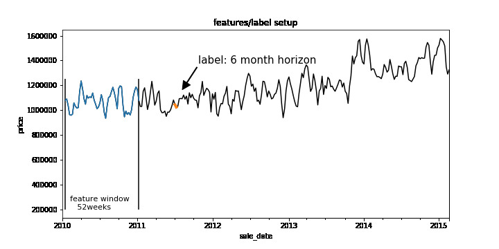
To create our features, we’ll pick a historical window size—e.g., one year—that will be used to forecast the median home price in six months. To do this, we have implemented a reusable function based on Pandas that allows you to easily generate time-series features and labels. Feel free to use this function on your own dataset.
After running create_rolling_features_label, a feature vector of length 52 (plus the date features) is created for each example, representing the features before the prediction date.
This can be shown with a rolling window:
Once we have the features and labels, the next step is to create a training and test set. In time-series problems, it’s important to split them temporally so that you are not leaking future information that would not be available at test time into the trained model.
In practice, you may want to scale your data using z-normalization or detrend your data to reduce seasonality effects. It may help to utilize differencing, as well to remove trend information. Now that we have features and labels, this simply becomes a traditional supervised learning problem, and you can use your favorite ML library to train a model. Here is a simple example using sklearn:
Scale our model
Let's imagine we want to put our model into production and automatically run it every week, using batch jobs, to get a better idea of future sales.Let’s also imagine we may want to forecast a model day-by-day.
Our data is stored in BigQuery, so let’s use the same logic that we used in Pandas to create features and labels, but instead run it at scale using BigQuery. We have developed a generalized Python function that creates a SQL string that lets you do this with BigQuery:
We pass the table name that contains our data, the value name that we are interested in, the window size (which is the input sequence length), the horizon of how far ahead in time we skip between our features and our labels, and the labels_size (which is the output sequence length). Labels size is equal to 1 here because, for now, we are only modeling sequence-to-one—even though this data pipeline can handle sequence-to-sequence. Feel free to write your own sequence-to-sequence model to take full advantage of the data pipeline!
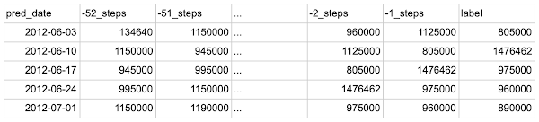
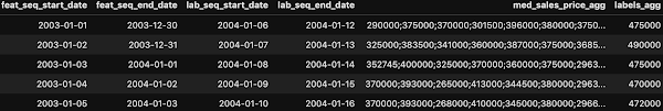
We can then execute the SQL stringscalable_time_series in BigQuery. A sample of the output shows that each row is a different sequence. For each sequence, we can see the time ranges of the features and the labels. For the features, the timespan is 52 weeks, which is the window_size, and for labels it is one day, which is the labels_size.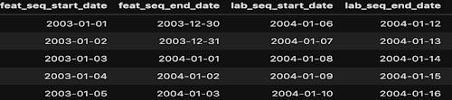
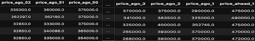
Looking at the same sampled rows, we can see how the training data is laid out. We have a column for each timestep of the previous price, starting with the farthest back in time on the left and moving forward. The last column is the label, the price one week ahead.
Now we have our data, ready for training, in a BigQuery table. Let’s take advantage of BigQuery ML and build a forecasting model using SQL.
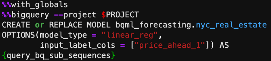
Above we are creating a linear regression model using our 52 past price features and predicting our label price_ahead_1. This will create a BQML MODEL in our bqml_forecasting dataset.
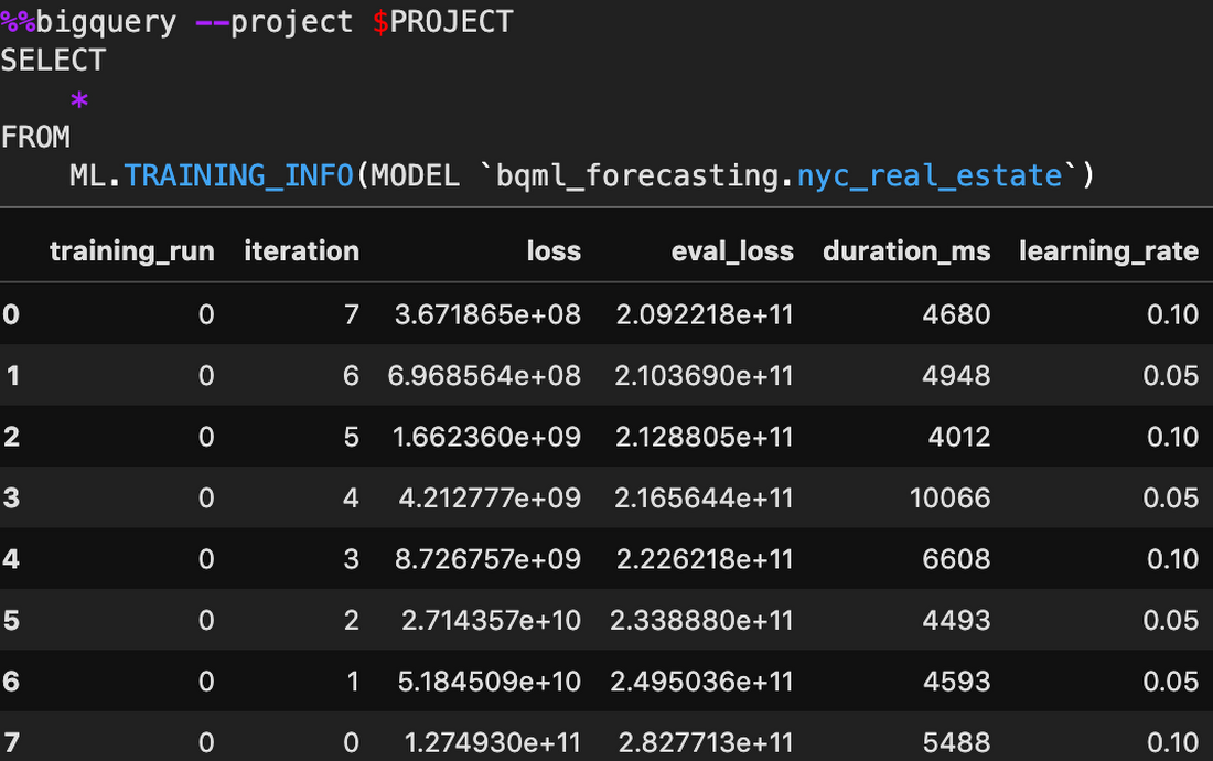
We can check how our model performed by calling TRAINING_INFO. This shows the training run index, iteration index, the training and eval loss at each iteration, the duration of the iteration, and the iteration's learning rate. Our model is training well since the eval loss is continually getting smaller for each iteration.
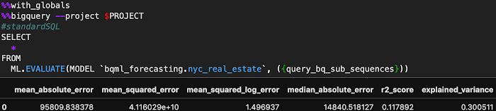
We can also do an evaluation of our trained model by calling EVALUATE. This will show common evaluation metrics that we can use to compare our model with other models to find the best choice among all of our options.
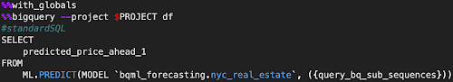
Lastly, machine learning is all about prediction. The training is just a means to an end. We can get our predictions by using the above query, where we have prepended predicted_ to the name of our label.
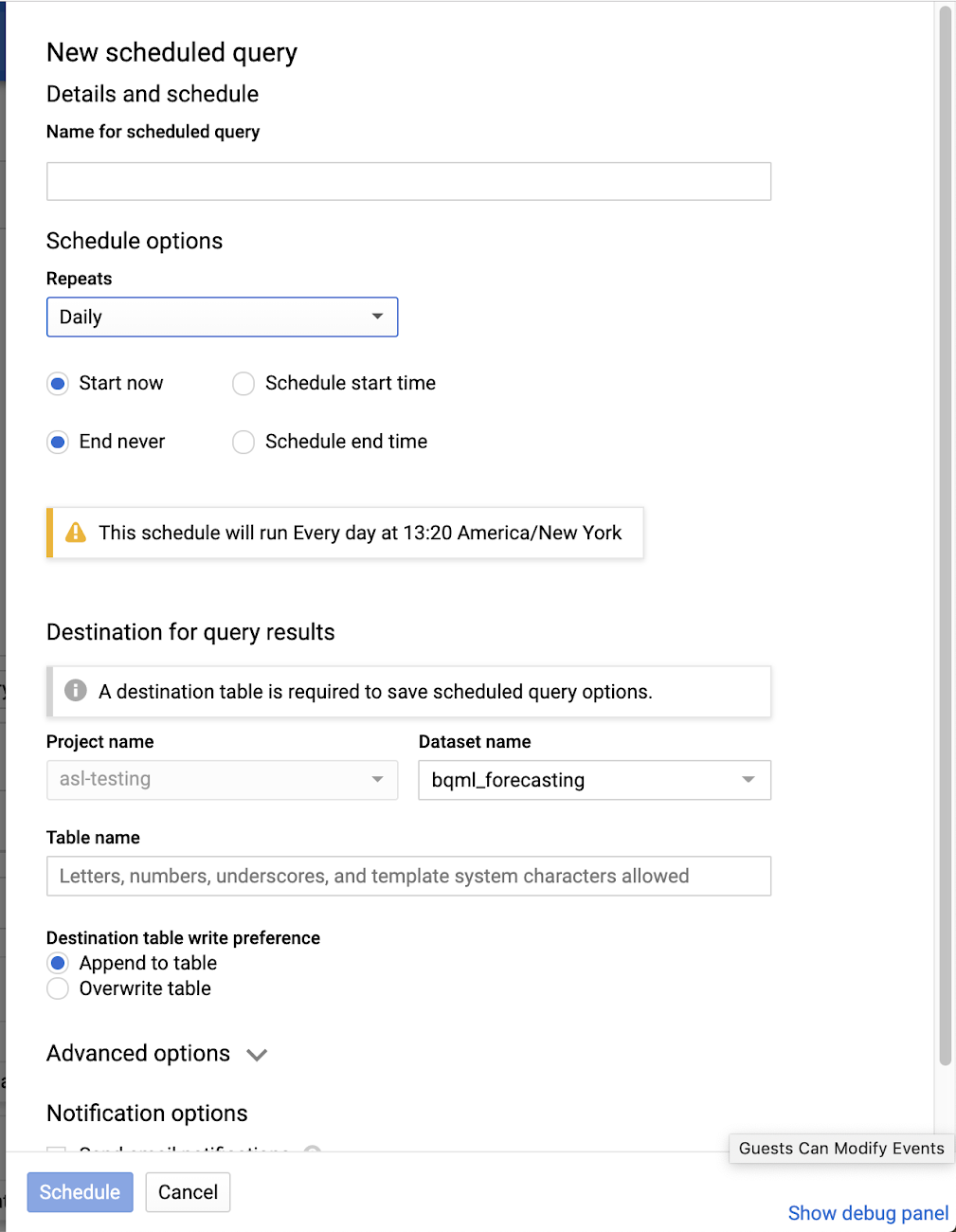
Now, let’s imagine that we want to run this model every week. We can easily create a batch job that is automatically executed using a scheduled query.
Of course, if we want to build a more custom model, we can use TensorFlow or another machine library, while using this same data engineering approach to create our features and labels to be read into our custom machine learning model. This technique could possibly improve performance.
To use an ML framework like TensorFlow, we'll need to write the model code and also get our data in the right format to be read into our model. We can make a slight modification to the previous query we used for BigQuery ML so that the data will be amenable to the CSV file format.
For this example, imagine you wanted to build a sequence-to-sequence model in TensorFlow that can handle variable length features. One approach to achieve this would be to aggregate all the features into a single column named med_sales_price_agg, separated by semicolons. The features (if we have more than just this feature in the future) and the label are all separated by a comma.
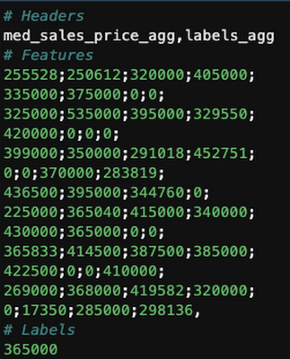
We'll execute the query in BigQuery and will make a table for train and eval. This will then get exported to CSV files in Cloud Storage. The diagram above is what one of the exported CSV files looks like—at least the header and the first line—with some comments added. Then when reading the data into our model using tf.data, we will specify the delimiter pattern shown above to correctly parse the data.
Please check out our notebook on AI Hub for an end-to-end example showing how this would work in practice and how to submit a training job on Google Cloud AI Platform. For model serving, the model can deployed on AI Platform or it can be deployed directly in BigQuery.
Conclusion
That's it! The workflow we shared will allow you to automatically and quickly setup any time-series forecasting problem. Of course, this framework can also be adapted for a classification problem, like using a customer’s historical behavior to predict the probability of churn or to identify anomalous behavior over time. Regardless of the model you build, these approaches let you quickly build an initial model locally, then scale to the cloud using BigQuery.
Learn more about BigQuery and AI Platform.