How to detect machine-learned anomalies in real-time foreign exchange data

Let's say you are a quantitative trader with access to real-time foreign exchange (forex) price data from your favorite market data provider. Perhaps you have a data partner subscription, or you're using a synthetic data generator to prove value first. You know there must be thousands of other quants out there with your same goal. How will you differentiate your anomaly detector?

What if, instead of training an anomaly detector on raw forex price data, you detected anomalies in an indicator that already provides generally agreed buy and sell signals? Relative Strength Index (RSI) is one such indicator; it is often said that RSI going above 70 is a sell signal, and RSI going below 30 is a buy signal. As this is just a simplified rule, it means there could be times when the signal is inaccurate, such as a currency market correction, making it a prime opportunity for an anomaly detector.

This gives us the following high level components:

Of course, we want each of these components to handle data in real time, and scale elastically as needed. Dataflow pipelines and Pub/Sub are the perfect services for this. All we need to do is write our components on top of the Apache Beam sdk, and they’ll have the benefit of distributed, resilient and scalable compute.

Luckily for us, there are some great existing Google plugins for Apache Beam. Namely, a Dataflow time-series sample library that includes RSI calculations, and a lot of other useful time series metrics; and a connector for using AI Platform or Vertex AI inference within a Dataflow pipeline. Let’s update our diagram to match, where the solid arrows represent Pub/Sub topics.

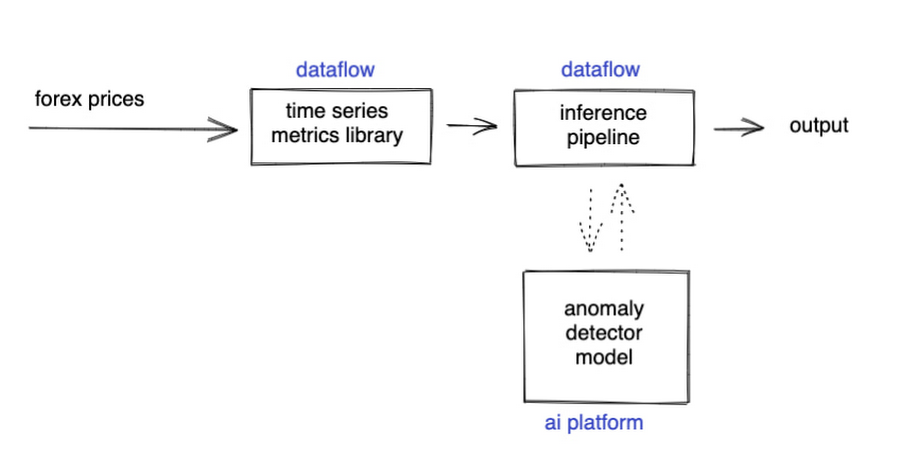
The Dataflow time-series sample library also provides us with gap-filling capabilities, which means we can rely on having contiguous data once the flow reaches our machine learning (ML) model. This lets us implement quite complex ML models, and means we have one less edge case to worry about.

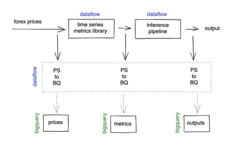
So far we’ve only talked about the real time data flow, but for visualization and continuous retraining of our ML model, we’re going to want historical data as well. Let’s use BigQuery as our data warehouse, and Dataflow to plumb Pub/Sub into it. As this plumbing job is embarrassingly parallelizable, we wrote our pipeline to be generic across data types and share the same Dataflow job, such that compute resources can be shared. This results in efficiencies of scale both in cost savings and time required to scale-up.

Data Modeling

Let’s discuss data formats a bit further here. An important aspect of running any data engineering project at scale is flexibility, interoperability and ease of debugging. As such, we opted to use flat JSON structures for each of our data types, because they are human readable and ubiquitously understood by tooling. As BigQuery understands them too, it’s easy to jump into the BigQuery console and confirm each component of the project is working as expected.

As you can see, the Dataflow sample library is able to generate many more metrics than RSI. It supports generating two types of metrics across time series windows, metrics which can be calculated on unordered windows, and metrics which require ordered windows, which the library refers to as Type 1 metrics and Type 2 metrics, respectively. Unordered metrics have a many-to-one relationship, which can help reduce the size of your data by reducing the frequency of points through time. Ordered metrics run on the outputs of the unordered metrics, and help to spread information through the time domain without loss in resolution. Be sure to check out the Dataflow sample library documentation for a comprehensive list of metrics supported out of the box.

As our output is going to be interpreted by our human quant, let’s use the unordered metrics to reduce the time resolution of our flow of real time data to one per second, or one hertz. If our output was being passed into an automated trading algorithm, we might choose a higher frequency. The decision for the size of our ordered metrics window is a little more difficult, but broadly determines the amount of time-steps our ML model will have for context, and therefore the window of time for which our anomaly detection will be relevant. We at least need it to be larger than our end-to-end latency, to ensure our quant will have time to act. Let’s set it to five minutes.

Data Visualization

Before we dive into our ML model, let’s work on visualization to give us a more intuitive feel for what’s happening with the metrics, and confirm everything we’ve got so far is working. We use the Grafana helm chart with the BigQuery plugin on a Google Kubernetes Engine (GKE) Autopilot cluster. The visualisation setup is entirely config-driven and provides out-of-the-box scaling, and GKE gives us a place to host some other components later on.

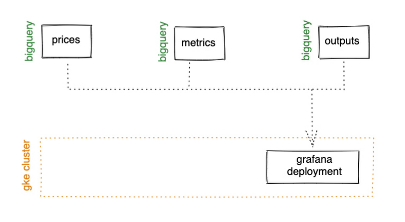
GKE Autopilot has Workload Identity enabled by default, which means we don’t need to worry about passing around secrets for BigQuery access, and can instead just create a GCP service account that has read access to BigQuery and assign it to our deployment through the linked Kubernetes service account.

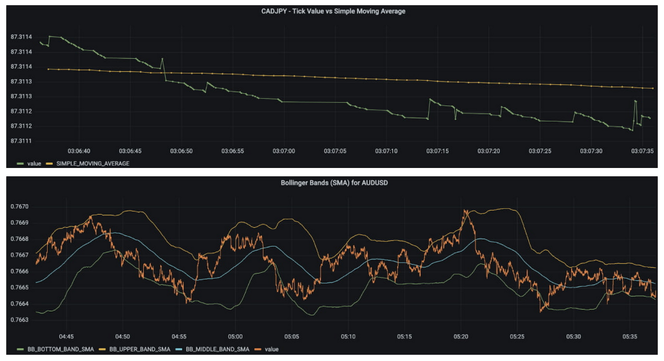
That’s it! We can now create some panels in a Grafana dashboard and see the gap filling and metrics working in real time.

Building and deploying the Machine Learning Model

Ok, ML time. As we alluded to earlier, we want to continuously retrain our ML model as new data becomes available, to ensure it remains up to date with the current trend of the market. TensorFlow Extended (TFX) is a platform for creating end-to-end machine learning pipelines in production, and eases the process around building a reusable training pipeline. It also has extensions for publishing to AI Platform or Vertex AI, and it can use Dataflow runners, which makes it a good fit for our architecture. The TFX pipeline still needs an orchestrator, so we can host that in a Kubernetes job, and if we wrap it in a scheduled job, then our retraining happens on a schedule too!

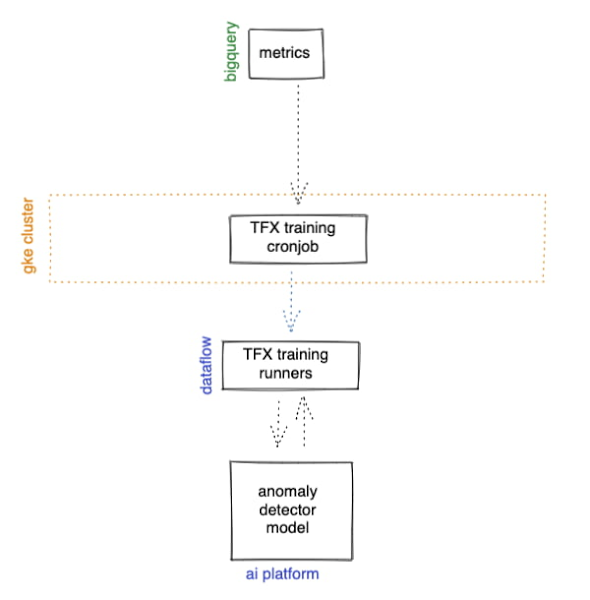
TFX requires our data be in the tf.Example format. The Dataflow sample library can output tf.Examples directly, but this tightly couples our two pipelines together. If we want to be able to run multiple ML models in parallel, or train new models on existing historical data, we need our pipelines to only be loosely coupled. Another option is to use the default TFX BigQuery adaptor, but this restricts us to each row in BigQuery mapping to exactly one ML sample, meaning we can’t use recurrent networks. 

As neither of the out-of-the-box solutions met our requirements, we decided to write a custom TFX component that did what we needed. Our custom TFX BigQuery adaptor enables us to keep our standard JSON data format in BigQuery and train recurrent networks, and it keeps our pipelines loosely coupled! We need the windowing logic to be the same for both training and inference time, so we built our custom TFX component using standard Beam components, such that the same code can be imported in both pipelines.

With our custom generator done, we can start designing our anomaly detection model. An autoencoder utilising long-short-term-memory (LSTM) is a good fit for our time-series use case. The autoencoder will try to reconstruct the sample input data, and we can then measure how close it gets. That difference is known as the reconstruction error. If there is a large enough error, we call that sample an anomaly. To learn more about autoencoders, please consider reading chapter 14 from Deep Learning by Ian Goodfellow, Yoshua Bengio, and Aaron Courville.

Our model uses simple moving average, exponential moving average, standard deviation, and log returns as input and output features. For both the encoder and decoder subnetworks, we have 2 layers of 30 time step LSTMs, with 32 and 16 neurons, respectively.

In our training pipeline, we include z score scaling as a preprocessing transformer - which is usually a good idea when it comes to ML. However, there’s a nuance to using an autoencoder for anomaly detection. We need not only the output of the model, but also the input, in order to calculate the reconstruction error. We’re able to do this by using model serving functions to ensure our model returns both the output and preprocessed input as part of its response. As TFX has out-of-the-box support for pushing trained models to AI Platform, all we need to do is configure the pusher, and our (re)training component is complete.

Detecting Anomalies in real time

Now that we have our model in Google Cloud AI Platform, we need our inference pipeline to call to it in real time. As our data is using standard JSON, we can easily apply our RSI rule of thumb inline, ensuring our model only runs when needed. Using the reconstructed output from AI Platform, we are then able to calculate the reconstruction error. We choose to stream this directly into Pub/Sub to enable us to dynamically apply an anomaly threshold when visualising, but if you had a static threshold you could apply it here too.

Summary

Here’s what the wider architecture looks like now:

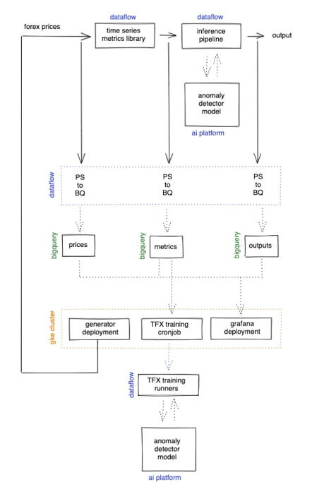
More importantly though, does it fit for our use case? We can plot the reconstruction error of our anomaly detector against the standard RSI buy/sell signal, and see when our model is telling us that perhaps we shouldn’t blindly trust our rule of thumb. Go get ‘em, quant!

In terms of next steps, there are many things you could do to extend or adapt what we’ve covered. You might want to explore with multi-currency models, where you could detect when the price action of correlated currencies is unexpected, or you could connect all of the Pub/Sub topics to a visualization tool to provide a real-time dashboard.

Give it a try

To finish it all off, and to enable you to clone the repo and set everything up in your own environment, we include a data synthesizer to generate forex data without needing access to a real exchange. As you might have guessed, we host this on our GKE cluster as well. There are a lot of other moving parts - TFX uses a SQL database and all of the application code is packaged into a docker image and deployed along with the infra using Terraform and cloud build. But if you’re interested in those nitty gritty details, head over to the repo and get cloning!

Feel free to reach out to our teams at Google Cloud and Kasna for help in making this pattern work best for your company.

^{Thank you very much to the Kasna and Google Cloud teams involved, particularly to Lucas Sargent (Kasna) and Reza Rokni (Google Cloud) for their outstanding contributions.}