BigQuery Admin reference guide: Query optimization

Last week in the BigQuery reference guide, we walked through query execution and how to leverage the query plan. This week, we’re going a bit deeper - covering more advanced queries and tactical optimization techniques.  Here, we’ll walk through some query concepts and describe techniques for optimizing related SQL. 

Filtering data

From last week’s post, you already know that the execution details for a query show us how much time is spent reading data (either from persistent storage, federated tables or from the memory shuffle) and writing data (either to the memory shuffle or to persistent storage). Limiting the amount of data that is used in the query, or returned to the next stage, can be instrumental in making the query faster and more efficient. 

Optimization techniques

1. Necessary columns only: Only select the columns necessary, especially in inner queries. SELECT * is cost inefficient and may also hurt performance. If the number of columns to return is large, consider using SELECT * EXCEPT to exclude unneeded columns.

2. Auto-pruning with partitions and clusters: Like we mentioned in our post on BigQuery storage, partitions and clusters are used to segment and order the data. Using a filter on columns that the data is partitioned or clustered on can drastically reduce the amount of data scanned. 

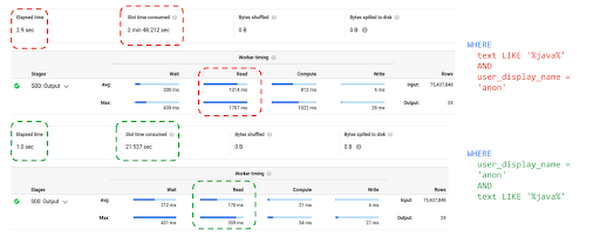
3. Expression order matters: BigQuery assumes that the user has provided the best order of expressions in the WHERE clause, and does not attempt to reorder expressions. Expressions in your WHERE clauses should be ordered with the most selective expression first.  The optimized example below is faster because it doesn’t execute the expensive LIKE expression on the entire column content, but rather only on the content from user, ‘anon’.

Understanding aggregation

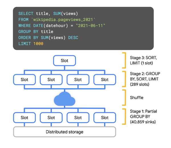
In an aggregation query, GROUP BYs are done in individual workers and then shuffled such that key value pairs of the same key are then in the same worker. Further aggregation then occurs and is passed into a single worker and served.

Repartitioning

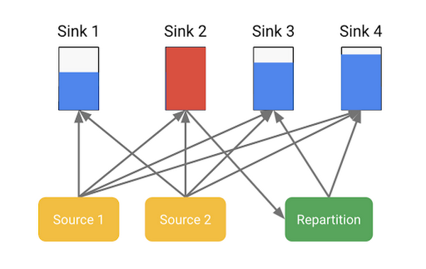
If too much data ends up on a single worker, BigQuery may re-partition the data. Let’s consider the example below. The sources start writing to Sink 1 and 2 (partitions within the memory shuffle tier). Next, the shuffle Monitor detects Sink 2 is over the limit. Now, the partitioning scheme changes and the sources stop writing to Sink 2, and instead start writing to Sink 3 and 4. 

Optimizations

For example, instead of a query like this, where you aggregate in both the subqueries and the final SELECT:

You should only aggregate once, in the outer query:

{order_id1, [ {item_id1}, {item_id2} ] }

Understanding joins

One powerful aspect of BigQuery is the ability to combine data, and understand relationships and correlation information from disparate sources. Much of the JOIN syntax is about expressing how that data should be combined, and how to handle data when information is mismatched. However, once that relationship is encoded, BigQuery still needs to execute it. 

Hash-based joins

Let's jump straight into large scale join execution.  When joining two tables on a common key, BigQuery favors a technique called the hash-based join, or more simply a hash join. With this technique, we can process a table using multiple workers, rather than moving data through a coordinating node.  

So what does hashing actually involve? When we hash values, we're converting the input value into a number that falls in a known range. There's many properties of hash functions we care about for hash joins, but the important ones are that our function is deterministic (the same input always yields the same output value) and has uniformity (our output values are evenly spread throughout the allowed range of values).

With an appropriate hashing function, we can then use the output to bucket values.  For example, if our hash function yields an output floating point value between 0 and 1, we can bucket by dividing that key range into N parts, where N is the number of buckets we want.  Grouping data based on this hash value means our buckets should have roughly the same number of discrete values, but even more importantly, all duplicate values should end up in the same bucket. 

Now that you understand what hashing does, let's talk through joining.

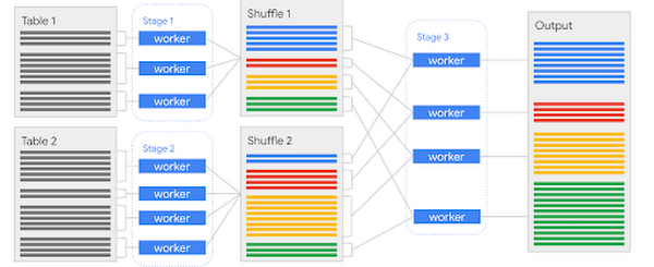
To perform the hash join, we're going to split up our work into three stages.

Stage 1: Prepare the first table

In BigQuery, data for a table is typically split into multiple columnar files, but within those files there's no sorting guarantee that ensures that the columns that represent the join key are sorted and colocated.  So, what we do is apply our hashing function to the join key, and based on the buckets we desire we can write rows into different shuffle partitions. 

In the diagram above, we have three columnar files in the first table, and we've using our hashing technique to split the data into four buckets (color coded).  Once the first stage is complete, the rows of the first table are effectively split into four "file-like" partitions in shuffle, with duplicates co-located.

Stage 2:  Prepare the second table

This is effectively the same work as the first stage, but we're processing the other table we'll be joining data against. The important thing to note here is that we need to use the same hashing function and therefore the same bucket grouping, as we're aligning data. In the diagram above, the second table had four input files (and thus four units of work), and the data was written into a second set of shuffle partitions.

Stage 3: consume the aligned data and perform the join

After the first two stages are completed, we've aligned the data in the two tables using a common hash function and bucketing strategy.  What this means is that we have a set of paired shuffle partitions that correspond to the same hash range, which means that rather than scanning potentially large sets of data, we can execute the join in pieces, as each worker is provided only the relevant data for doing it's subset of the join.

It's at this point that we care about the nature of the join operation again; depending on the desired join relationship we may yield no rows, a single row, or many rows for any particular input row from the original input tables.

Now, you can also get a better sense of how important having a good hashing function may be:  if the output values are poorly distributed, we have problems because we're much more likely to have a single worker that's slower and forced to do the majority of the work.  Similarly, if we picked our number of buckets poorly, we may have issues due to having split the work too finely or too coarsely.  Fortunately, these are not insurmountable problems, as we can leverage dynamic planning to fix this: we simply insert query stages to adjust the shuffle partitions.

Broadcast joins

Hash-based joins are an incredibly powerful technique for joining lots of data, but your data isn't always large enough to warrant it.  For cases where one of the tables is small, we can avoid all the alignment work altogether.

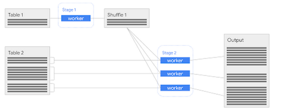
Broadcast joins work in cases where one table is small.  In these instances, it's easiest to replicate the small table into shuffle for faster access, and then simply provide a reference to that data for each worker that's responsible for processing the other table's input files.

Optimization techniques

1. Largest table first:  BigQuery best practice is to manually place the largest table first, followed by the smallest, and then by decreasing size. Only under specific table conditions does BigQuery automatically reorder/optimize based on table size.
2. Filter before joins: WHERE clauses should be executed as soon as possible, especially within joins, so the tables to be joined are as small as possible. We recommend reviewing the query execution details to see if filtering is happening as early as possible, and either fix the condition or use a subquery to filter in advance of a JOIN.
3. Pre-aggregate to limit table size: As mentioned above, aggregating tables before they are joined can help improve performance - but only if the amount of data being joined is drastically reduced and tables are aggregated to the same level (i.e., if there is only one row for every join key value).
4. Clustering on join keys: When you cluster a table based on the key that is used to join, the data is already co-located which makes it easier for workers to split the data into the necessary partitions within the memory shuffle. 

A detailed query: finding popular libraries in Github

Now that we understand some optimization techniques for filtering, aggregating and joining data - let’s look at a complex query with multiple SQL techniques. Walking through the execution details for this query should help you understand how data flows and mutates as it moves through the query plan - so that you can apply this knowledge and understand what’s happening behind the scenes in your own complex query.  

The public Github data has one table that contains information about source code filenames, while another contains the contents of these files.  By combining the two together, we can filter down to focus on interesting files and analyze them to understand which libraries are frequently used by developers. Here's an example of a query that does this for developers using the Go programming language. It scans files having the appropriate (.go) extensions, and looks for statements in the source code for importing libraries, then counts how often those libraries are used and how many distinct code repositories use them.

In SQL, it looks like this:

We can see from a casual read that we've got lots of interesting bits here: subqueries, both a distributed join (the contents and files tables), array manipulation (cross join unnest), and powerful features such as regular expression filters and computing distinctness.

Detailed stages and steps

First, let's examine the full details of the plan in a graph format.  Here, we're looking at the low level details of how this query is run, as a set of stages.  Let's work through the query stages in detail. If you want a graphical representation similar to the one we’re showing here, check out this code sample!

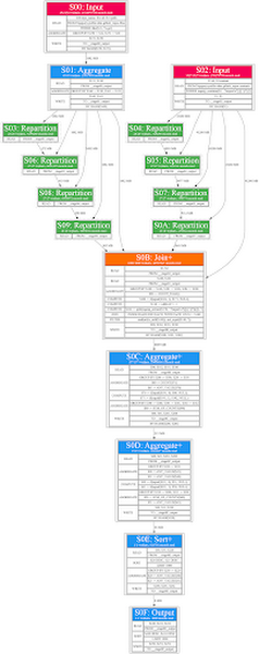
Stage S00-S01: Reading and filtering from the "files" table

The initial stage (corresponding to the inner subquery of the SQL) begins by processing the "files" table.  We can see the first task is to read the input, and immediately filter that to only pass through files with the appropriate suffix.  We then group based on the id and and repo name, as we're potentially working with many duplicates, and we only want to process each distinct pair once. In stage S01, we continue the GROUP BY operation; each worker in the first stage only deduplicated the repo/id pairs in their individual input file(s), the aggregate stage here is to combine those so that we've deduplicated across all input rows in the "files" table.

Stage S02: Reading in the "contents" table

In this stage, we begin reading the source code in the "contents" table, looking for "import" statements (the syntax for referencing libraries in the Go language).  We collect information about the id (which will become the join key), and the content which has matches. You can also see that in both this stage and the previous (S01), the output is split based on a BY HASH operation.  This is the first part of starting the hash join, where we begin to align join keys into distinct shuffle partitions.  However, anytime we're dealing with data where we want to divide the work we'll be splitting it into shuffle buckets with this operation.

Stages S03 - S0A: Repartitioning

This query invoked several repartitioning stages.  This is an example of the dynamic planner rebalancing data as it's working through the execution graph.  Much of the internals of picking appropriate bucketing is based on heuristics, as operations such as filtration can drastically change the amount of data flowing in and out of query stages. In this particular query, the query plan has chosen a non-optimal bucketing strategy, and is rebalancing the work as it goes.  Also note that this partitioning is happening on both sides of what will become the joined data, because we need to keep the partitioned data aligned as we enter the join.

Stage S0B: Executing the join

Here's where we begin correlating the data between the two inputs.  You can see in this stage we have two input reads (one for each side of the join), and start computing counts.  There's also some overloaded work here; we consume the file contents to yield an array representing each individual library being imported, and make that available to future stages.

Stages S0C - S0D: Partial Aggregations

These two stages are responsible for computing our top level statistics:  we wanted to count the total number of times each library was referenced, as well as the number of distinct repositories.  We end up splitting that into two stages.

Stage S0E-S0F: Ordering and limiting

Our query requested only the top 1000 libraries ordered first by distinct repository count, and then total frequency of use.  The last two stages are responsible for doing this sorting and reduction to yield the final result.

Other optimization techniques

As a final thought, we’ll leave you with a few more optimization techniques that could help improve the performance of your queries.

1. Multiple WITH clauses: The WITH statement in BigQuery is like a Macro. At runtime the contents of the subquery will be inlined every place the alias is referenced. This can lead to query plan explosion as seen by the plan executing the same query stages multiple times. Instead, try using a TEMP table.
2. String comparisons: REGEXP_CONTAINS can offer more functionality, but it has a slower execution time compare to LIKE. Make LIKE when the full power of regex is not needed (e.g. wildcard matching): 

regexp_contains(dim1, ‘.*test.*’) to dim1 like %test%

First or last record: When trying to calculate the first or last record in a subset of your data, using the ROW_NUMBER() function can fail with Resources Exceeded errors if there are too many elements to ORDER BY in a single partition. Instead, try using ARRAY_AGG() - which runs more efficiently because the ORDER BY is allowed to drop everything except the top record on each GROUP BY. For example, this:

Becomes this:

See you next week!

Thanks again for tuning in this week! Next up is data governance, so be sure to keep an eye out for more in this series by following Leigha on LinkedIn and Twitter.