Streaming analytics now simpler, more cost-effective in Cloud Dataflow

Streaming analytics helps businesses to understand their customers in real time and adjust their offerings and actions to better serve customer needs. It’s an important part of modern data analytics, and can open up possibilities for faster decisions. For streaming analytics projects to be successful, the tools have to be easy to use, familiar, and cost-effective. Since its launch in 2015, Cloud Dataflow, Google’s fully managed streaming analytics service, has been known for its powerful API available in Java and Python. Businesses have almost unlimited customization capabilities for their streaming pipelines when they use these two languages, but these capabilities come at the cost of needing programming skills that are sometimes hard to find.

To advance Google Cloud’s streaming analytics further, we’re announcing new features available in the public preview for Cloud Dataflow SQL, as well as the general availability of Cloud Dataflow Flexible Resource Scheduling (FlexRS) for a very cost-effective way of batch processing of events. These new features make streaming analytics easier and more accessible to data engineers, particularly those with database experience. 

Here’s more detail about each of these new features:

Cloud Dataflow SQL to create streaming (and batch) pipelines using SQL
We know that SQL is the standard for defining data transformations, and that you want more GUI-based tools for creating pipelines. With that in mind, several months ago we launched a public preview of Cloud Dataflow SQL, an easy way to use SQL queries to develop and run Cloud Dataflow jobs from the BigQuery web UI. Today, we are launching several new features in Cloud Dataflow SQL, including Cloud Storage file support and a visual schema editor.

Cloud Dataflow SQL allows you to join Cloud Pub/Sub streams with BigQuery tables and Cloud Storage files. It also provides several additional features:

• Using Streaming SQL extensions for defining time windows and calculating window-based statistics;

• Integration with Cloud Data Catalog for storing the schema of Cloud Pub/Sub topics and Cloud Storage file sets—a key enabler for using SQL with streaming messages;

• A simple-to-use graphical editor available in the BigQuery web UI. If you are familiar with BigQuery’s SQL editor, you can create Cloud Dataflow SQL jobs. 

To switch the BigQuery web UI to Cloud Dataflow SQL editing mode, open the BigQuery web UI, go to More>Query settings and select “Cloud Dataflow” as the query engine.

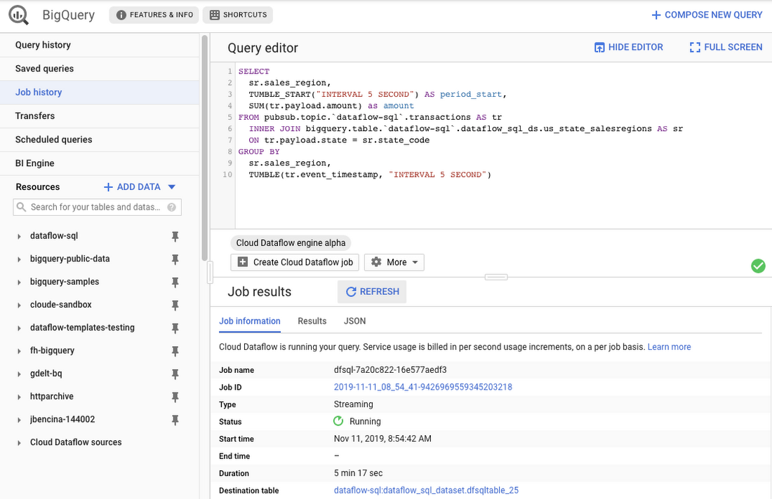
As an example, let’s say you have a Cloud Pub/Sub stream of sales transactions, and you want to build a real-time dashboard for the sales managers of your organization showing them the up-to-date stats of the sales in their regions. You can accomplish this in a few steps: write a SQL statement like the following one, launch a Cloud Dataflow SQL job, direct the output to a BigQuery table, then use one of the many supported dashboarding tools, including Google Sheets, Data Studio, and others, to visualize the results.

In this example, we are joining the “transactions” Cloud Pub/Sub topic in the “dataflow-sql” project with a metadata table in BigQuery called “us_state_salesregions.” This table contains a mapping between the state codes (present in the “transactions” Cloud Pub/Sub topic) and the sales regions “Region_1”, “Region_2”, .., “Region_N” that are relevant to the sales managers in our example organization. In addition to the join, we’ll do a streaming aggregation of our data, using one of the several windowing functions supported by Cloud Dataflow. In our case, we will use TUMBLE windows, which will divide our stream into fixed five-second time intervals, group all the data in those time windows by the sales_region field, and calculate the sum of sales in the sales region. We also want to preserve the start of each time window, via TUMBLE_START("INTERVAL 5 SECOND"), to plot sales amounts as a time series. 

To start a Cloud Dataflow job, click on “Create Cloud Dataflow job” in the BigQuery web UI.

When data starts flowing into the destination table, it will contain three fields: the sales_region, the timestamp of the period start, and the amount of sales. 

In the next step, we will create a BigQuery Connected Sheet that shows a column chart of sales in “Region_1” over time. Select the destination BigQuery table in the nav tree. In our case, it’s the dfsqltable_25 table.

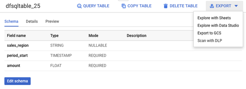
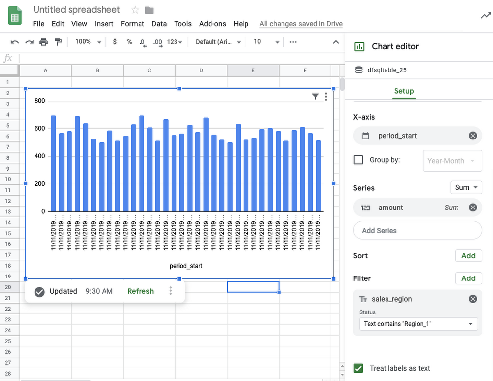
Then, select Export>Explore with Sheets to chart your data. Do it from the tab where your BigQuery table is shown, and not from the tab where your original Cloud Dataflow SQL was. In Sheets, create the column chart using the data connection to BigQuery, and choose period_start for the X-axis, amount as your data series, and add a sales_region filter. This is all you have to do to build a chart in Sheets that visualizes streaming data.

Mixing and joining data in Cloud Pub/Sub and BigQuery helps solve many real-time dashboarding cases, but quite a few customers have also asked for support of their Cloud Storage files to join those files with events in Cloud Pub/Sub or with tables in BigQuery. This is now possible in Dataflow SQL, enabled by our integration with Data Catalog’s Cloud Storage file sets. 

In the following example, you’ll see an archive of transactions stored in CSV files in the “transactions_archive” Cloud Storage bucket.

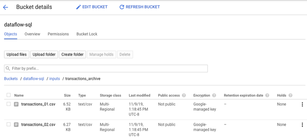
Two gcloud commands can define a Cloud Storage file set and entry group in Data Catalog.

Notice how we defined the file pattern “gs://dataflow-sql/inputs/transactions_archive/*.csv” as part of the file set entry definition. This pattern is what will allow Cloud Dataflow to find the CSV files once we write the SQL statement that references this file set.

We can even specify the schema of this transactions_archive_fs file set using a GUI editor. For that, go to the BigQuery web UI (make sure it is running in Cloud Dataflow mode), select “Add Data” in the left navigation and choose “Cloud Dataflow sources.” Search for your newly added Cloud Storage file set and add it to your active datasets in the BigQuery UI.

This will allow you to edit the schema of your file set after you select it in the nav tree. The “Edit schema” button is right there on the “Schema” tab. The visual schema editor is new and works for both Cloud Storage file sets as well as for Cloud Pub/Sub topics.

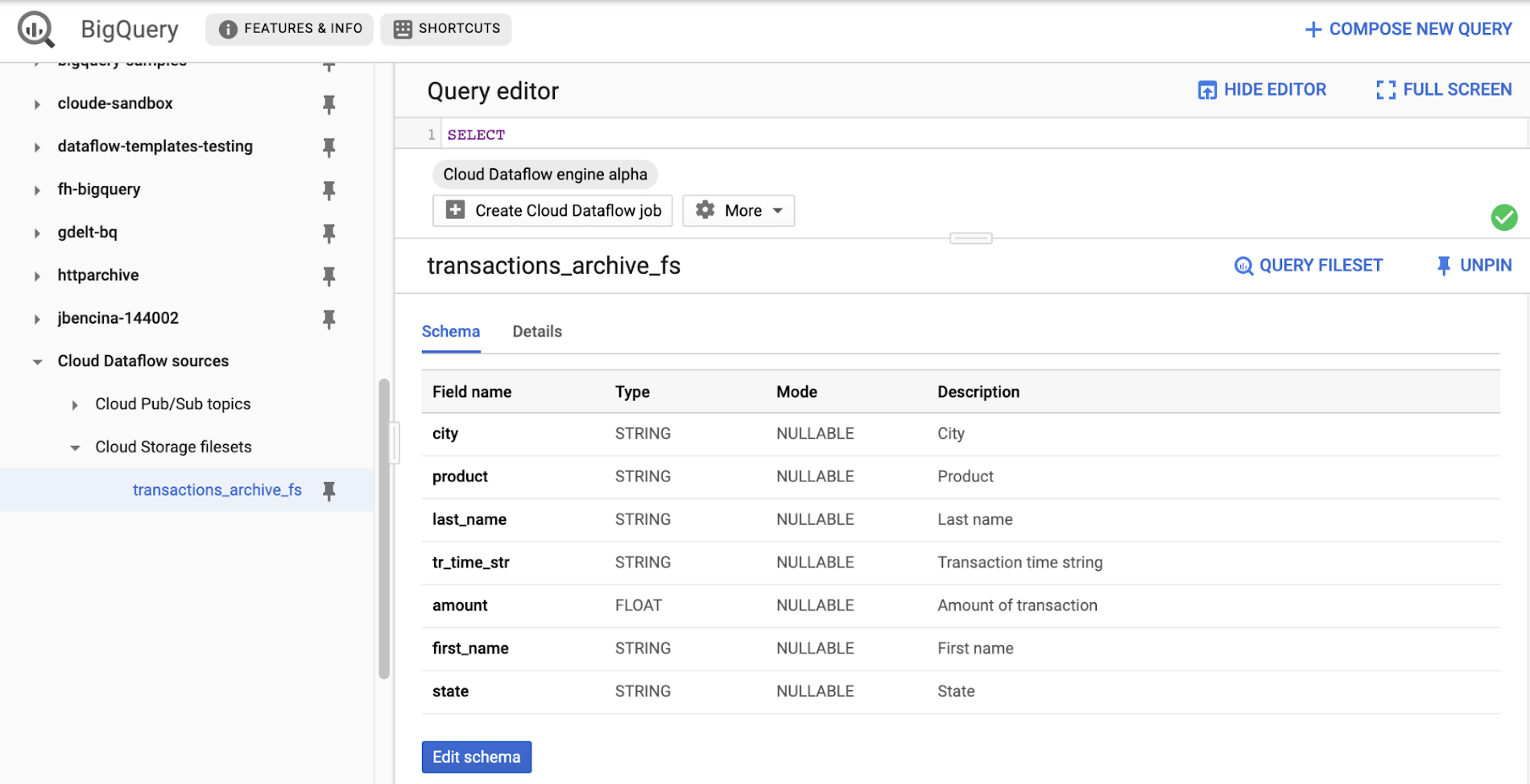
Once you’ve registered the file set in Data Catalog and defined a schema for it, you can query it in Cloud Dataflow SQL. In the next example, we’ll join the transactions archive in Cloud Storage with the metadata mapping table in BigQuery.

Notice how similar this SQL statement is to the one that queries Cloud Pub/Sub. The TUMBLE window function even works on Cloud Storage files, although we will define the windows based on a field “tr_time_str” that is inside the files (the Cloud Pub/Sub SQL statement used the tr.event_timestamp attribute of the Cloud Pub/Sub stream). The only other difference is the reference to the Cloud Storage file set. We accomplish this by specifying datacatalog.entry.`dataflow-sql`.`us-central1`.transactions_archive_eg.transactions_archive_fs AS tr

Because both of the job inputs are bounded (batch) sources, Cloud Dataflow SQL will create a batch job (instead of a streaming job created for the first SQL statement using a Cloud Pub/Sub source) which will join your Cloud Storage files with the BigQuery table, and write the results back to BigQuery.

And now you have both a streaming pipeline feeding your real-time dashboard from a Cloud Pub/Sub topic, as well as a batch pipeline capable of onboarding historical data from CSV files. Check out the SQL Pipelines tutorial to start applying your SQL skills for developing streaming (and batch) Cloud Dataflow pipelines.

FlexRS for cost-effective batch processing of events
While real-time streaming processing is an exciting use case that’s growing rapidly, many streaming practitioners know that every stream processing system needs a sprinkle of batch processing (as you saw in the SQL example). When you bootstrap a streaming pipeline, you usually need to onboard historical data, and this data tends to reside in files stored in Cloud Storage. When streaming events need to be reprocessed due to changes in business logic (i.e., time windows get readjusted, or new fields are added), this reprocessing is also better done in batch mode.

The Apache Beam SDK and the Cloud Dataflow managed service are well-known in the industry for their unified API approach to batch and streaming analytics. The same Cloud Dataflow code can run in either mode with just minimal changes (usually replacing the data source from Cloud Pub/Sub to Cloud Storage). Remember our SQL example, where switching the SQL statement from a streaming source to a batch source was no trouble at all? And while it’s easy to go back and forth between streaming and batch processing in Cloud Dataflow, an important factor influencing the processing choice is cost. Customers who gravitate to batch processing have always looked to find the right balance between the speed of execution and costs. In many cases, that may mean you can be flexible with the amount of time it takes to process a dataset if the overall cost of processing is reduced in a significant fashion. 

Our new Cloud Dataflow FlexRS feature reduces batch processing costs by up to 40% using advanced resource scheduling techniques and a mix of different virtual machine (VM) types (including the preemptible VM instances) to decrease processing costs while providing the same job completion guarantees as regular Cloud Dataflow jobs. FlexRS uses the Cloud Dataflow Shuffle service, which allows it to handle the preemption of worker VMs better because the Cloud Dataflow service does not have to redistribute unprocessed data to the remaining workers.

Using FlexRS requires no code changes in your pipeline and can be accomplished by simply specifying the following pipeline parameter:

--flexRSGoal=COST_OPTIMIZED

Running Cloud Dataflow jobs with FlexRS requires autoscaling, a regional endpoint in the intended region, and specific machine types, so you should review the recommendations for other pipeline settings. While Cloud Dataflow SQL does not yet support FlexRS, it will in the future.

Simultaneously with launching FlexRS in general availability, we are also extending its availability to five additional regions, covering all regions now where we have regional endpoints and Cloud Dataflow Shuffle:

• us-central1
• us-east1
• us-west1
• europe-west1
• europe-west4
• asia-east1
• asia-northeast1

To learn more about Cloud Dataflow SQL, check out our tutorial and try creating your SQL pipeline using the BigQuery web UI. Visit our documentation site for additional FlexRS usage and pricing information.

Check out other recently launched streaming and batch processing features: 

• We deployed Cloud Dataflow Shuffle and Cloud Dataflow Streaming Engine to three additional regions, bringing total availability to seven regions.

• We launched the ability to protect your pipeline state with customer-managed encryption keys.

Python streaming support from Cloud Dataflow is now generally available.