Introducing Cloud Dataflow’s new Streaming Engine
Sergei Sokolenko
Cloud Dataflow Product Manager
Many of our customers benefit from the design principle of separating compute from state storage used by Google in several Big Data services such as BigQuery and, most recently, in batch Cloud Dataflow pipelines using the Dataflow Shuffle. Today, we are launching Cloud Dataflow Streaming Engine in beta, to apply the same principle to streaming pipelines.
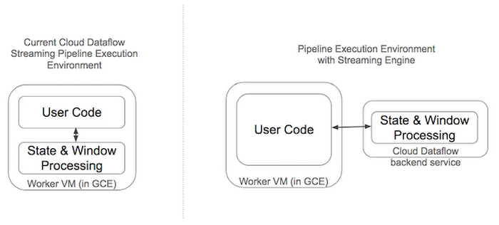
Almost every streaming Cloud Dataflow pipeline needs to shuffle data and store time window state. Currently, Cloud Dataflow performs these operations on worker Virtual Machines and uses attached Persistent Disks for window state and shuffle storage. The new opt-in Streaming Engine (also now available in beta) moves these operations from worker VMs into a Cloud Dataflow backend service, leading to several improvements:
- More responsive autoscaling in response to incoming data volume variation. The Streaming Engine offers smoother, more granular worker scaling.
- Reductions in consumed worker VM resources (CPU, memory, and Persistent Disk storage). The Streaming Engine works best with smaller worker machine types (
n1-standard-2instead ofn1-standard-4) and does not require Persistent Disk beyond a small worker boot disk. - Improved supportability, since users don’t need to re-deploy their pipelines to apply service updates
Streaming autoscaling improvements
Consider a workload that processes a stream of events with a data rate that varies throughout the day. For example, this workload could ingest events from smart devices, join them with metadata, calculate averages over a pre-defined time window, and store the enriched events and statistics into BigQuery for further analysis. The following figure shows the rates of input data in an illustrative workload. It varies anywhere from a couple of million bytes per second to more than 10 million bytes per second.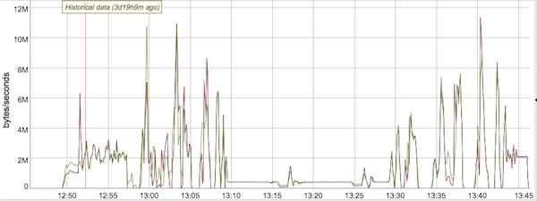
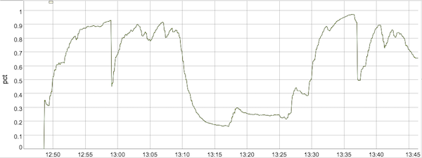
In the current Dataflow streaming architecture that does not use the Streaming Engine, Dataflow would observe the CPU utilization of worker VMs and, once it becomes sufficiently high, would autoscale the number of workers to a higher value. In the graph in Figure 3 this occurred about 9 minutes into the job, at 12:57pm, when Dataflow autoscaled from 3 workers all the way up to 15 workers. As the inbound data rate remained high, the CPU utilization of workers also stayed high, justifying the continued deployment of 15 workers. Then, around 1:10pm, the inbound data rate declined significantly, and after a short 6 minute delay to make sure that more data was not still inbound, Dataflow downscaled first to 8 workers and then to 5 workers. Just as Dataflow scaled down to 5 workers, our inbound data rate picked up again, and Dataflow reacted after observing the CPU utilization by increasing the number of workers again to 15 at the 1:35 pm mark, where it stayed until the end of this job.
In our new streaming architecture, where the Streaming Engine is responsible for state storage and streaming shuffle, the same input data stream would result in a similar autoscaling decision at 9-minute time mark (see graph below). However, streaming pipelines using the Streaming Engine do not need quite as many workers to accomplish the same work, so Dataflow autoscaled to 13 workers (and not 15, as before). Furthermore, Dataflow downscaled much more quickly (after 3 minutes instead of 6 minutes) and to a lower number of workers (first 5, and then 3, instead of 8 and 5 as before), when the first streaming data wave ended.
Review the changes of active workers with and without Streaming Engine in Figures 3 and 4.
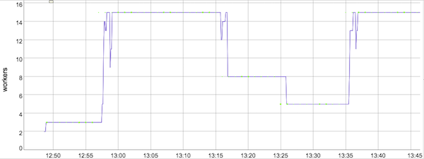
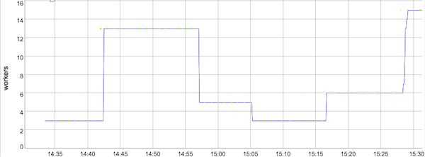
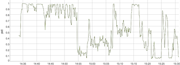
When the second wave of streaming data came, the Streaming Engine adjusted workers upwards in several steps, matching the increase in input rate, and saving resources. If you look at the purple plot in Figure 4 starting at time 15:15, Dataflow scaled from 6 workers to 7, then 8 (you need to look closer for this one, as it happened very quickly), then 13, 14, and finally reached 15. Compare this to the auto-scaling behaviour without the Streaming Engine (see Figure 3), where Dataflow oscillated for a few minutes between 5 and 15 workers, going up and down several times.
Overall, worker resource usage with the Streaming Engine, visualized by the area below the purple Active Workers graph, was significantly lower than without the Streaming Engine. Also, autoscaling was much more sensitive to the inbound data rate, resulting in quicker scaling up and down of workers. Review the Pricing section of the blog for information on additional charges associated with the use of the Streaming Engine.
You can review and compare the worker CPU utilization, aggregated over all workers, with and without Streaming Engine in Figures 5 and 6. The rise in CPU utilization due to the increase in incoming data that we mentioned earlier is clearly visible in graphs between time marks 12:50 to 12:57 (Figure 5) and 14:34 to 14:42 (Figure 6). This rise in CPU utilization gives the signal to the Dataflow autoscaler to add more workers. You can also see how CPU utilization drops initially after the active workers scale up (the pipeline gets more CPUs then) at time mark 12:57 (Figure 5), but then starts to climb because the input data rate also continues to increase. The added resources are being used efficiently to handle the new data load.
Enabling Streaming Engine and best practices
Dataflow users don’t have to change any of their pipeline code to take advantage of the new architecture for shuffle and window state processing. During Streaming Engine beta they can simply use a pipeline parameter to opt into using the Streaming Engine, and, after the feature is released into General Availability, Streaming Engine will be turned on by default for all new streaming pipelines.One of the biggest benefits of the Steaming Engine is a much improved autoscaling capability. By default, when you specify the --experiments=enable_streaming_engine parameter, we will enable autoscaling automatically. You have the option of disabling autoscaling by specifying the --autoscalingAlgorithm=NONE parameter, but we do not recommend you do that.
Streaming Engine provides the most resource savings with worker machine types that are smaller than the default streaming workers, using by default n1-standard-2 workers instead of n1-standard-4. If your streaming pipelines use a different worker type than n1-standard-4, try a worker that is about half as large as what you are currently using (e.g. n1-standard-4 to replace n1-standard-8) by specifying --workerMachineType=<your-machine-type>.
Monitoring usage
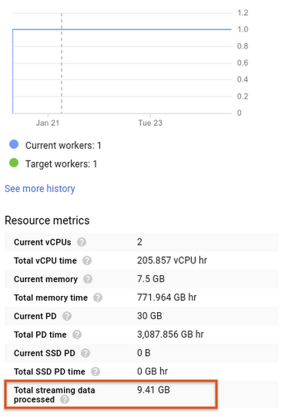
You can observe the volume of streaming data processed both in the Dataflow Job Details page as well as in Stackdriver Monitoring.In the Dataflow Job Details page (Cloud Console > Dataflow > then, select a particular job), every job that runs with the Streaming Engine (see below for how to enable it) will show you an extra metric representing the total processed volume. In the example below, the total data processed was 9.41 GB.
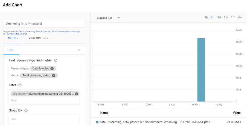
When you navigate to Stackdriver Monitoring, GCP’s monitoring service, you can chart this metric in custom Dashboards, and even define alerts when this metric’s growth exceeds predefined thresholds, or drops below a healthy value. Go to Stackdriver Monitoring > Dashboards > Create Dashboard, and select Add Chart. Then, in the Chart pane, look for Dataflow Job resource type, and select the Total streaming data processed metric. If you want to review a particular job, specify a filter and set the Job Name or Job ID. The figure below shows the graph for a single streaming job that used about 21 MB of Streaming Data Processed.
Early success with alpha customers
During our alpha program, many customers had the chance to try out their streaming pipelines with the new Streaming Engine. Here are some early reports from their successful implementations:The Dataflow Streaming Engine, enabled with just a single parameter and without any code changes in our streaming pipeline, has helped us realize a much better distribution of load and autoscaling. In terms of ROI for the effort this is probably the biggest bang for the buck. Simple, efficient and just works! It’s quintessentially Google
—Ankur Chauhan, Software Engineer, Brightcove
We at Vente-Exclusive.com really love Cloud Dataflow to run our Beam pipelines. Google is constantly innovating, and as a Google Cloud Platform customer, we didn’t have to change a single line of code to run on the new Streaming Engine. Our streaming pipeline processes real-time events ingested over Pub/Sub and stores the processed results in Bigtable. It ran without any issues for several months—that’s fire-and-forget real-time processing!
—Alex Van Boxel, Big Data Architect at Vente-Exclusive.com
Pricing
Reductions in worker resources and downsizing of worker machine types are enabled by offloading the shuffling and state processing work from worker VMs to a Cloud Dataflow backend service. For that reason, there is a charge associated with the use of the Streaming Engine. Streaming Engine is billed by the amount of streaming data processed by it (the pricing unit is also called “Streaming Data Processed”). Each GB of Streaming Data Processed is priced at $0.018.While costs of pipelines using the Streaming Engine will vary somewhat from the costs of pipelines not using this feature, when you look at your total bill for streaming Cloud Dataflow pipelines and consider different streaming usage patterns, we expect the bill to remain approximately the same as before, when aggregated over all your streaming use cases.
This Streaming Data Processed volume depends on how much data you ingested into your streaming pipeline and the complexity and number of fused pipeline stages. Examples of what counts as a Streaming Data Processed include data inflows from data sources, flows of data from one fused pipeline stage to another fused stage, flows of data persisted in user-defined state or used for windowing, and data outflows to data sinks, such as Pub/Sub or BigQuery.
Getting started
Cloud Dataflow Streaming Engine is currently in beta and you can opt-in to using it by specifying an experiments parameter.- Use the
--experiments=enable_streaming_engineparameter to opt-in your Dataflow streaming job - Specify one of the two GCP regions supported at beta (us-central1 or europe-west1) by using the
--region={ us-central1 | europe-west1 }parameter. More regions will follow - Dataflow Streaming Engine is available in pipelines using the Java SDK; support for pipelines using the Python SDK will be added in the future.