From raw data to machine learning model, no coding required
Karl Weinmeister
Director, Developer Relations
Machine learning was once the domain of specialized researchers, with complex models and proprietary code required to build a solution. But, Cloud AutoML has made machine learning more accessible than ever before. By automating the model building process, users can create highly performant models with minimal machine learning expertise (and time).
However, many AutoML tutorials and how-to guides assume that a well-curated dataset is already in place. In reality, though, the steps required to pre-process the data and perform feature engineering can be just as complicated as building the model. The goal of this post is to show you how to connect all the dots, starting with real-world raw data and ending with a trained model.
Use case
Our goal will be to predict the monthly average incident response time for the Fire Department of New York (FDNY). We’ll start by downloading historical data from 2009-2018 from the NYC OpenData website as a CSV.
The dataset has 4,368 rows, each with the average response time for that month. The data is partitioned by the incident type (False Alarm, Medical Emergency, etc.), borough, and the number of incidents during that month.
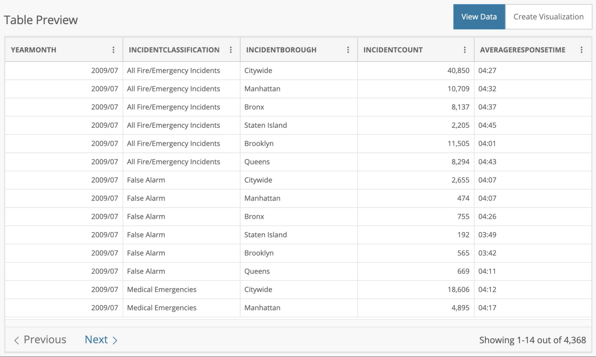
Notice that the column we'd like to predict, AVERAGERESPONSETIME, is in a mm:ss format. We'll need to change that into a numeric format, such as seconds. This is an example of a processing step on the raw data that is required to build a model.
Getting started
We'll be working with four products in this post:
Cloud Storage: the storage service our raw data is stored in
Cloud Data Fusion: the data integration service that will orchestrate our data pipeline
BigQuery: the data warehouse that will store the processed data
AutoML Tables: the service that automatically builds and deploys a machine learning model
The first step is to upload the CSV file into a Cloud Storage bucket so it can be used in the pipeline. Next, you'll want to create an instance of Cloud Data Fusion. Follow the first two steps in the documentation to enable the API and create an instance.
In BigQuery, you'll need to create a table within a new or existing dataset. There’s no need to create a schema; we'll do that automatically in our data pipeline. Let's get started with the pipeline.
Creating the data pipeline
Cloud Data Fusion enables you to build a scalable data integration pipeline for batch or real-time scenarios. You can design the pipeline with UI components that represent standard data sources and transformations. The pipeline is then executed as MapReduce, Spark, or Spark Streaming programs on a Dataproc cluster.
Our pipeline will consist of three steps:
Retrieving the CSV file from Cloud Storage
Transforming the data into a format that is suitable for machine learning
Storing the processed data in a BigQuery table
To get started, click on the Studio view to create a new pipeline. We’ll walk through each step of the pipeline illustrated here.
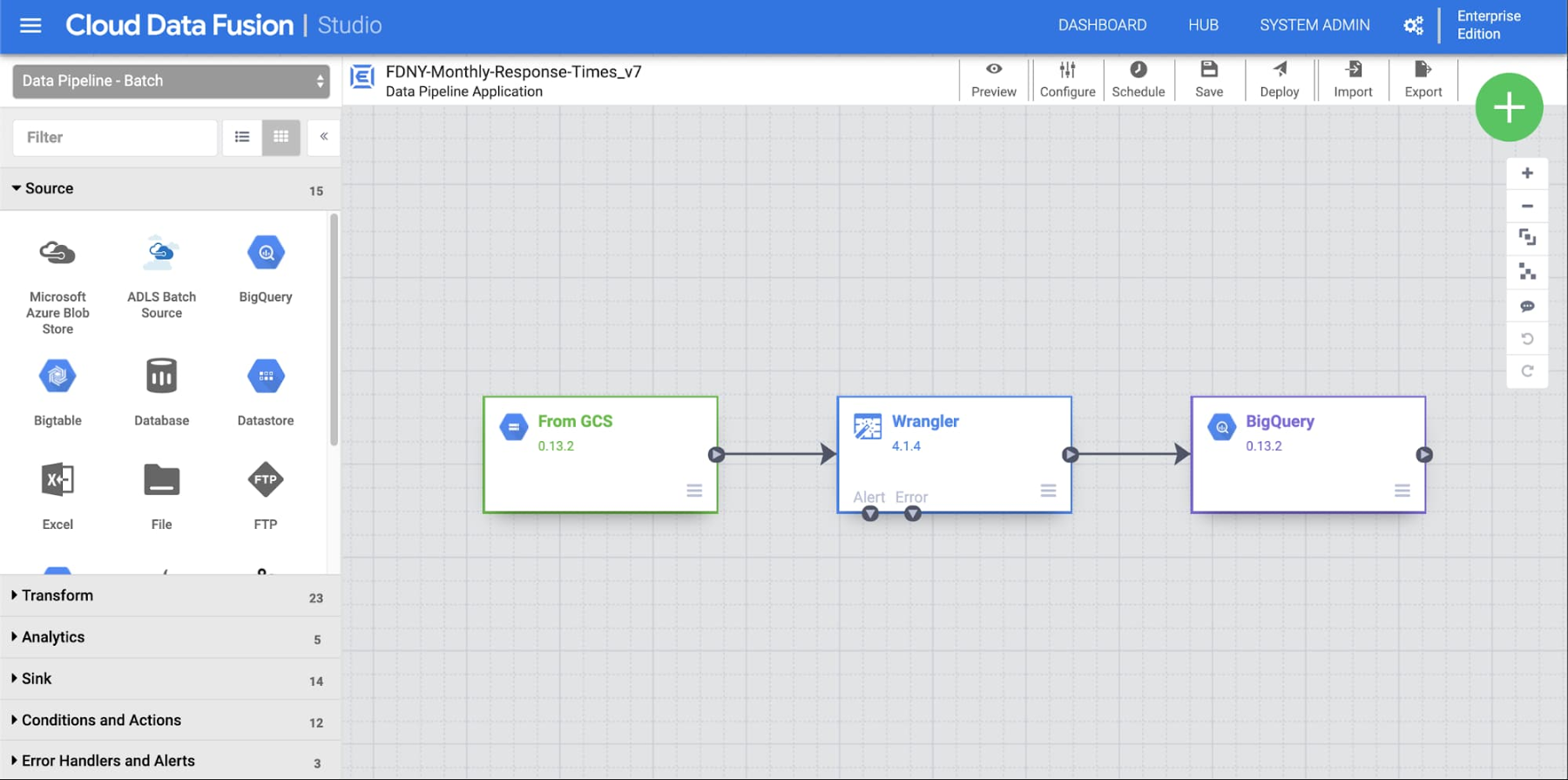
You can drag and drop each node, or plugin, to the canvas and connect them. Let's start with the input node. From the list of Source plugins, add a new GCS plugin to the canvas, then update its properties. Feel free to use your own label and reference name, and make sure that the path matches the location of your CSV file:
- Label: From GCS
- Reference Name: GCS1
- Path: gs://<YOUR_BUCKET>/FDNY_Monthly_Response_Times.csv
Transforming the data
Next, we'll transform the data using the Wrangler plugin—a powerful component that contains a suite of parsing, transformation, and mapping utilities to perform common tasks with data.
From the list of Transform plugins, add a Wrangler plugin and connect its input to the output of "From GCS." You can use whatever label you'd like, such as "FDNY Response Time Wrangler."
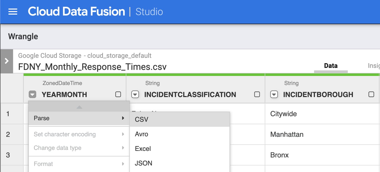
Click Wrangle and navigate to the CSV in the storage bucket. Then click the arrow next to body and select Parse -> CSV, with these options set:
- Separate by comma
- Check the box "Set first row as header"
Following a similar process as you did in the parse step, follow these additional steps to complete the transformations:
Parse YEARMONTH as a Simple date
Use custom format: yyyy/MM
Filter out All Incidents under INCIDENTCLASSIFICATION
Filter -> Remove Rows - > Value is "All Fire/Emergency Incidents"
Filter out Citywide under INCIDENTBOROUGH
Filter -> Remove Rows -> Value is "Citywide"
Delete columns body and INCIDENTCOUNT
We don't know the number of incidents prior to the month beginning
Remove the colon from AVERAGERESPONSETIME by:
Find and replace ":" with "" (no quotes)
Convert AVERAGERESPONSETIME to seconds with:
Custom transform: (AVERAGERESPONSETIME / 100) * 60 + (AVERAGERESPONSETIME % 100)
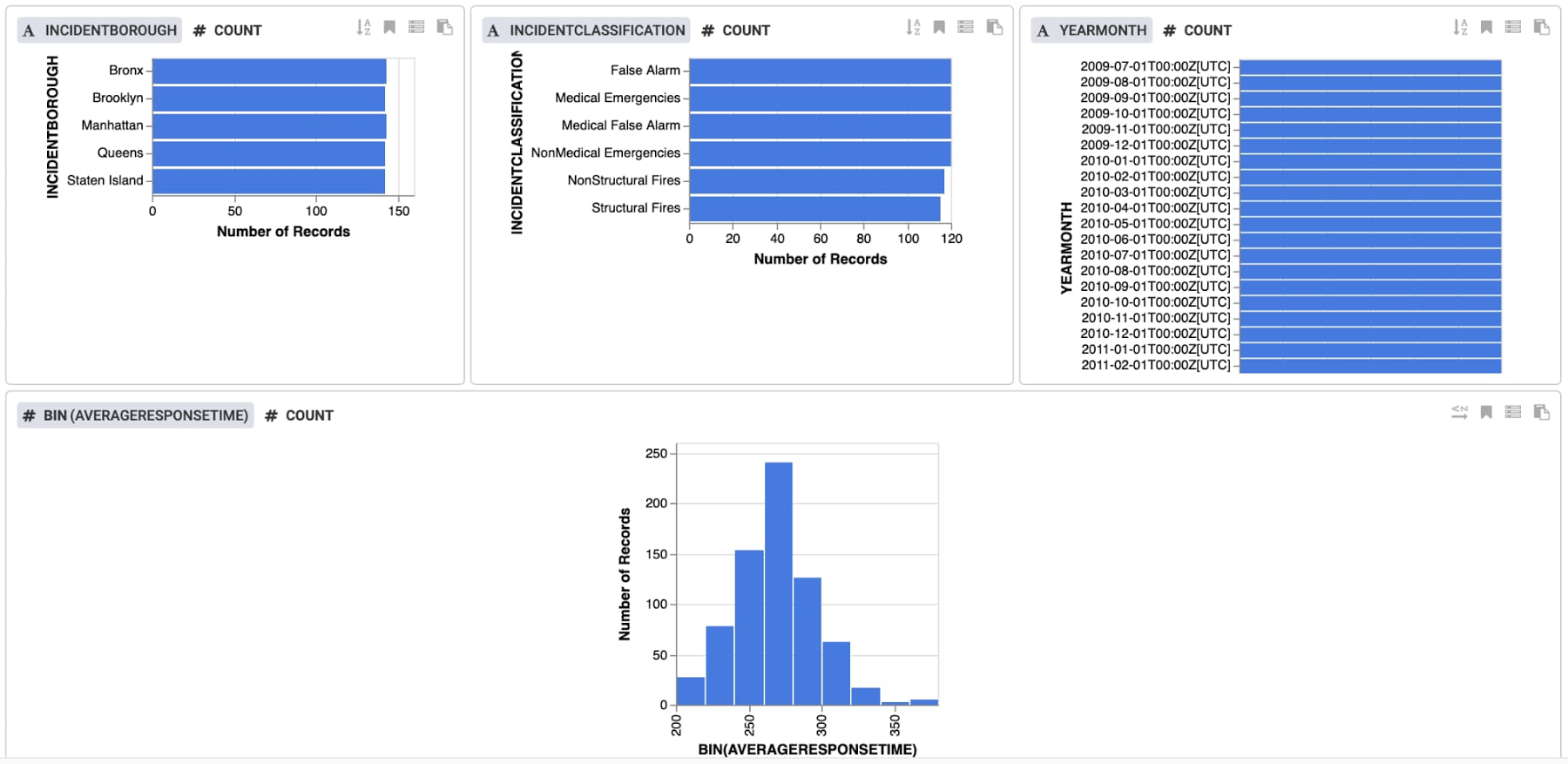
Click Insights near the top to review the data in more detail. Views are provided for each column, and you can also create custom views. The data indicates that there is a good balance of values for each feature, and we see a normal distribution of response times, centered around 270 seconds.
Click to Apply the transformations, and then click to Validate the plugin. You should see "No Errors" shown.
Storing the data in BigQuery
The final step of the pipeline will be to write each record into the BigQuery table. We'll set the Update Table Schema option in the BigQuery plugin, so that each data field name and type will be automatically populated in BigQuery.
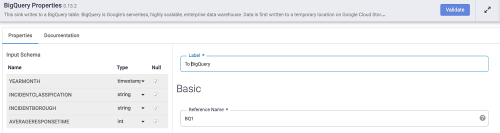
From the link of Sink plugins, add BigQuery to the canvas. Then, click Properties to set the fields as follows:Label: To BigQuery
Reference Name: BQ1
Dataset: <YOUR_DATASET>
Table: <YOUR_NAME>
Update Table Schema: True
Click Validate to ensure that your plugin is configured correctly.
Deploying and running the pipeline
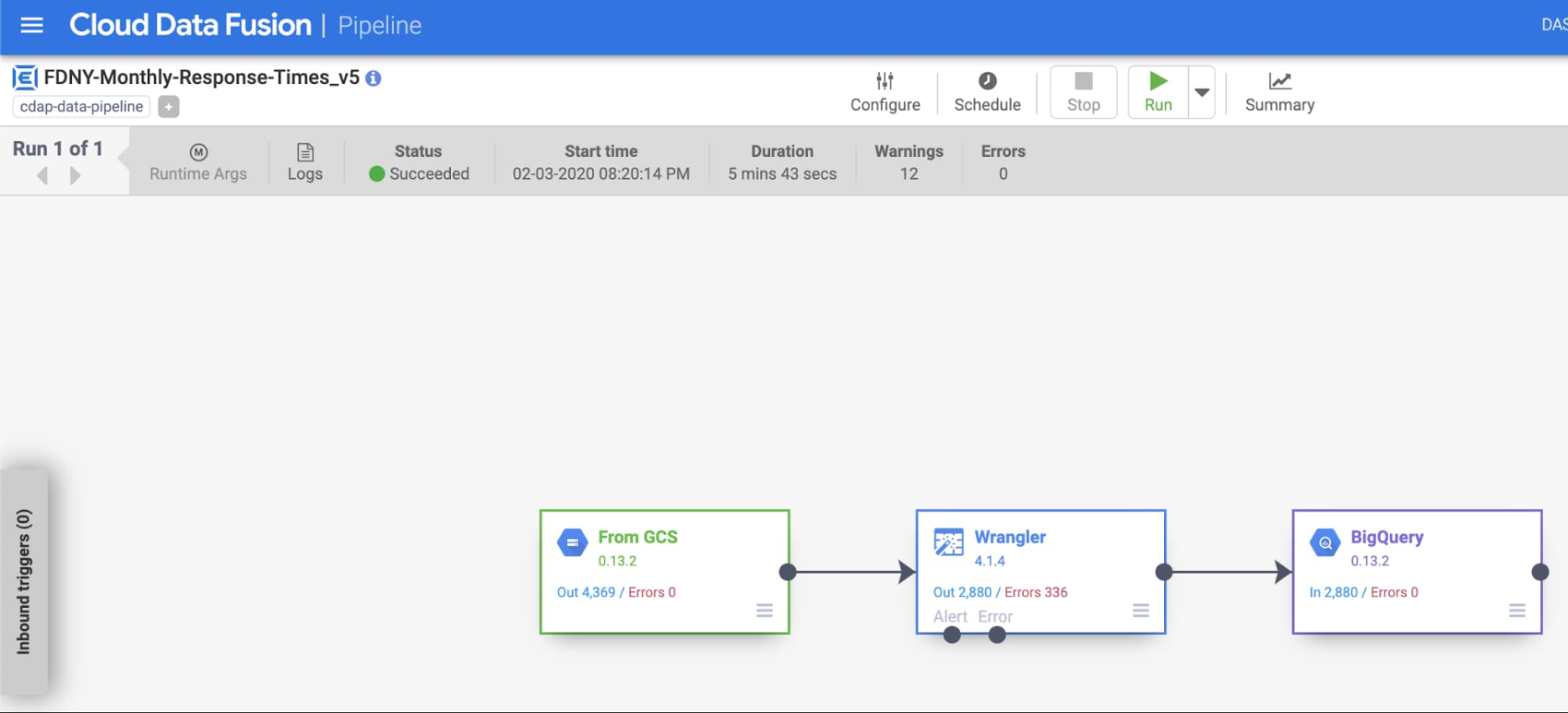
With our data transformed and in BigQuery, we're ready to deploy the pipeline. In the top menu bar, name the pipeline something like fdny_monthly_response_time and save it. Next, deploy the pipeline, which will take about a minute. Finally, you're ready to run the pipeline. This step will take several minutes to provision a Dataproc cluster and run.
By default, Cloud Data Fusion will create an ephemeral cluster to execute the pipeline, and will delete the cluster when finished. You can also choose to run the pipeline on an existing cluster. As the job proceeds, you can see information such as the status, duration, and errors.
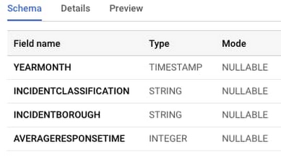
Review the transformed data in BigQuery
While you could skip ahead to directly import your model in AutoML Tables, it never hurts to review the output of the transformation. Access the BigQuery console and navigate to the table you've created. Click Schema to see what was created for you by the pipeline:
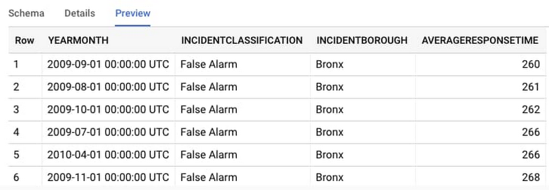
Then, click Preview to see some example rows from the dataset:
Build a model with AutoML Tables
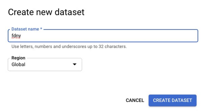
The data looks good, so now it's time to create a model! Access AutoML Tables and start by creating a new dataset.
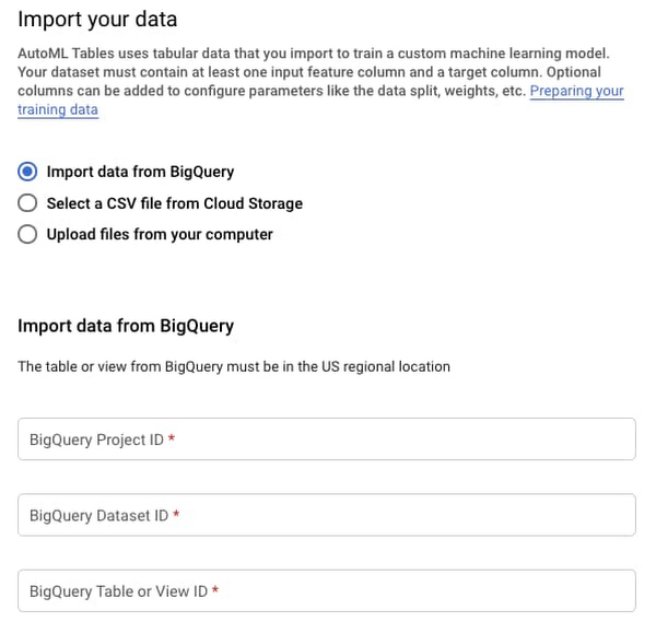
From there, you will need to import the data into your model. It's straightforward to directly import data from BigQuery: Simply provide the Project ID, Dataset ID, and Table Name, and then import the data.
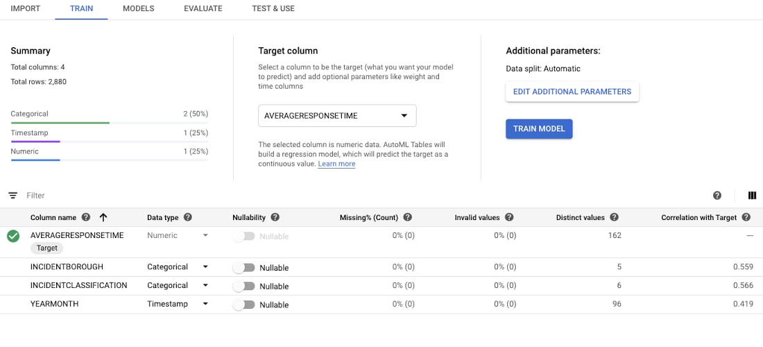
After you’ve imported the data, you can begin training. There's only one option you have to set, which is your Target column, or the variable you're aiming to predict. You will be predicting a numeric value, so you’ll be creating a regression model. AutoML also supports classification models, which are used to predict which category the input belongs to. AutoML Tables should infer the data types and the standard settings, such as an 80/10/10 Train/Test/Validate split, are fine as-is. Select AVERAGERESPONSETIME or the target column.
After selecting the target column, AutoML Tables will recompute statistics about each model feature. You can then select Train Model.
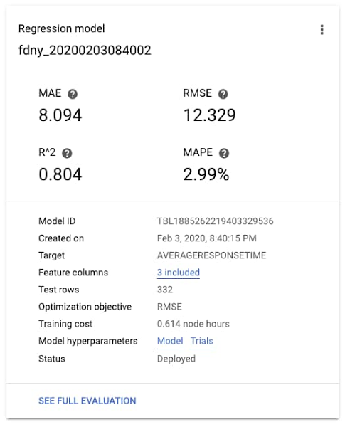
After some time, training will complete and you can review the accuracy statistics for your model. In this case, the MAE (Mean Absolute Error) is about 8 seconds, and the R2, or the variance explained by the model—which ranges from 0-1—is about 0.8. Not bad!
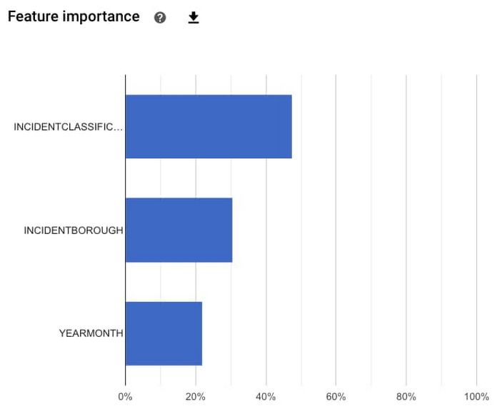
You can also see which features had the most predictive power in the model. In this case, it looks like the most important feature was the type of incident, then the borough in which the incident occurred, and finally the time of the year. The feature importances provided here are calculated across the entire test dataset, to understand the general magnitude of impact. We'll see later that you can find out feature importances for a specific prediction.
Finally, you can try predicting with your model. There are a few options available: batch prediction, online prediction, and model export as a Docker container.
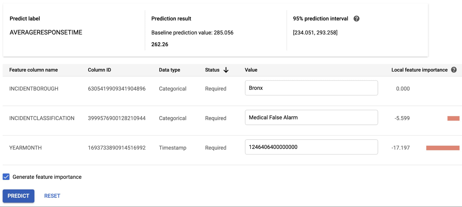
Let's try an online prediction. After deploying your model, you can access it as a REST API. The AutoML Tables user interface provides a handy way to test this API. Let's enter some test values. (Note the YEARMONTH field is a Unix timestamp in microseconds. For example, 1246406400000000 in the table below is midnight on July 1, 2009.) You can see a prediction result of 262.26 seconds! You also see that YEARMONTH had the largest impact on this particular prediction.
Wrapping it up
In this post, you've seen that it’s possible to build a robust pipeline and ML model without coding. Under the hood, each step of the process is realized by scalable infrastructure. The pipeline runs on a cloud native Dataproc cluster and inserts records into a scalable BigQuery data warehouse. We then run a neural architecture search in AutoML Tables to build a model.
And, remember, we didn’t start with a squeaky clean dataset, either. Being able to transform less-than-perfect data to something your model can use opens up machine learning to even more use cases. So, whatever your use case is, enjoy your next experience working with these powerful tools.