Monitor & analyze BigQuery performance using Information Schema

In the exponentially growing data warehousing space, it is very important to capture, process and analyze the metadata and metrics of the jobs/queries for the purposes of auditing, tracking, performance tuning, capacity planning, etc. 

Historically, on-premise (on-prem) legacy data warehouse solutions have  mature methods  of collecting and reporting performance insights  via query log reports, workload repositories etc.  However all of this comes with an overhead of cost-storage & cpu.

To give customers easy access and visibility to BigQuery metadata and metrics, Google Cloud launched Information Schema in 2020. The Information Schema gives customers a lens to consume the metadata and performance indicators for every BigQuery job/query/API.  The storage associated with the Information Schema Views is free.  Users only pay for the cost of the Compute associated with analyzing this information. 

There are multiple factors that contribute to BigQuery spend. The two most common are storage and processing (querying), which also tend to be the largest items on your bill at the end of the month. 

In this blog, we will equip you with an easy way to analyze and decipher the key BigQuery metrics using the Information Schema.

Before getting started, it is important to understand the concept of a “slot” in BigQuery. For the purpose of this blog, we will be looking at the “Jobs Metadata by TimeSlice” view in the Information Schema. More on the Information Schema views here. 

In this blog we’ll look at a couple of use cases.

• Analyze BigQuery Slot Consumption and  Concurrency for a Point in Time

• Analyze Query Throughput and % Busy for a Time Period

One important highlight is to note the difference between “Concurrent Query Count” and “Query Throughput Count”.  

• “Concurrent Query Count” represents the actual number of queries running at a specific point in time.  

• “Query Count” which is often used to describe the number of queries running over some interval of time.  

The ultimate goal of this exercise is to produce a result set that we can export to Google Sheets and drop into a Pivot Table. We can then create visualizations for slot consumption and concurrency. This is critically important as it pertains to:

1. “Right-sizing” reservation allocations

2. Understanding the impact of newly introduced workloads into your environment

3. Determining if workloads are relying on idle slot capacity in order to meet SLAs

4. Proactively identifying trends which might ultimately result in concurrency limit errors

Alternatively, you can run this from Google Sheets using the BigQuery connector. The queries and charting will be similar in either case.

In short, we will use this information to optimize spend while ensuring consistently for the workloads that need it most.

Also, a couple of key points to remember and act on for both the below scripts:

• Change the ‘Region’ qualifier of the Information Schema if you aren’t part of the ‘region-US’. For example, if your datasets are in us-east4, change the qualifier to ‘us-east4’. i.e region-us-east4.INFORMATION_SCHEMA.JOBS_TIMELINE_BY_PROJECT

• In the BigQuery Console/ UI, under More→Query Settings→ Additional Settings, change the Data Location to the location where your dataset is residing. For example, if your datasets are in us-east4, select that region.

Analyze / visualize point in time slot consumption and concurrency

The purpose of this query is to collect information for all the jobs that are running during a range of time, broken into smaller intervals in which we will capture a single second (Point In Time).  

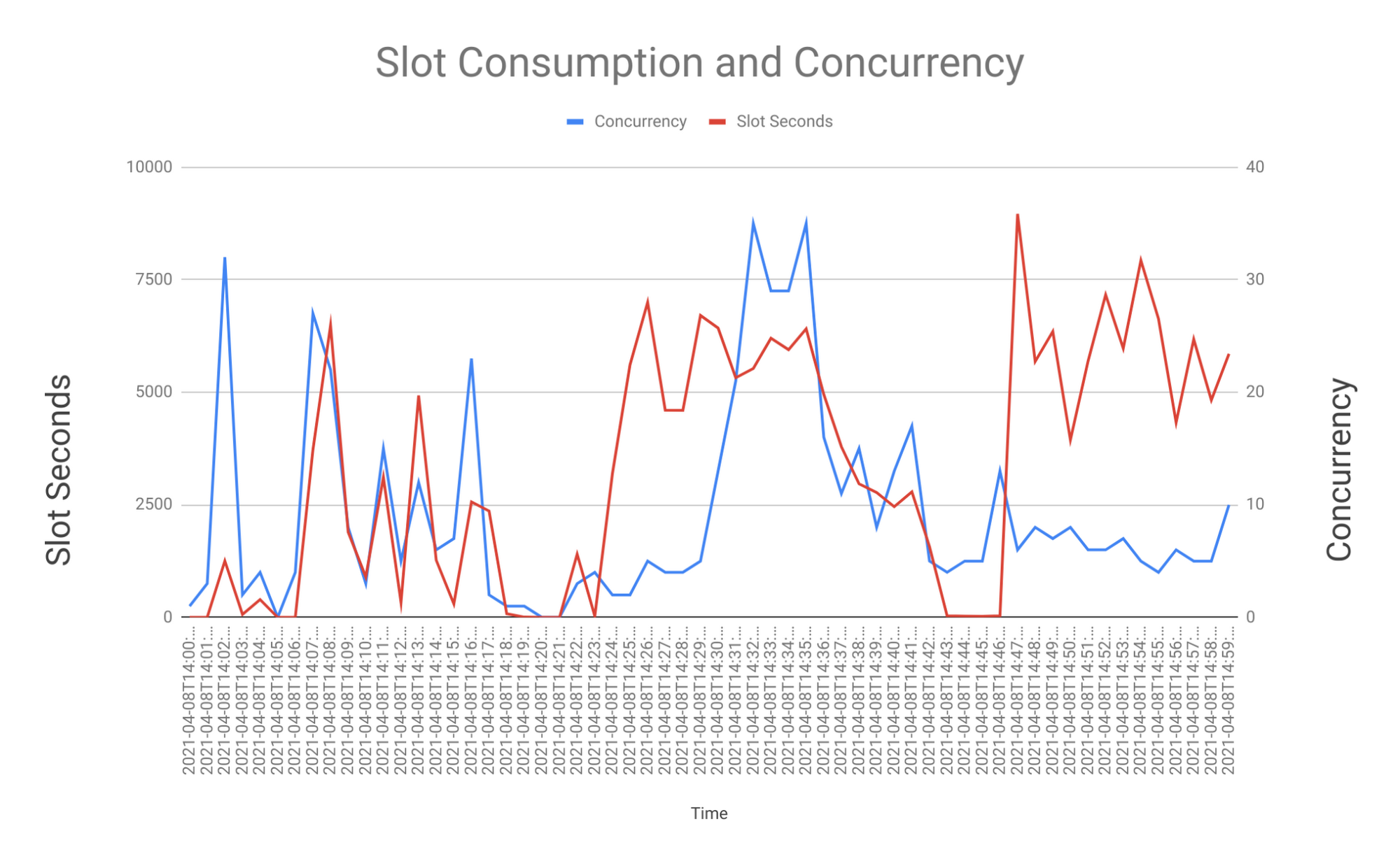
The final charts used to visualize this data will have Time on the X-Axis. For the Y-Axis, we will either have Slot Seconds or Concurrent Query Count...or, we can have both with a Primary and Secondary Y-Axis defined.  

Main SQL

Here is the SQL script from the github repo, copy-paste into the BigQuery UI and run it!  

Let's break down the SQL into smaller chunks for easy understanding.

Declaring and setting variables

We will be declaring 7 variables.  

As you can see, these variables are all related to time. After declaring, it is time to set these variables. 

Let's set the values for the 7 declared variables.  The first 4 variables will need to be set manually by the individual running the query.  

• The first variable (_TIMEZONE) should represent your local TimeZone.  

• The second (_RANGE_START_TS_LOCAL) and third (_RANGE_END_TS_LOCAL) variables will represent the range of time using your local TimeZone which you want to analyze.  

• The fourth variable (_RANGE_INTERVAL_SECONDS) represents the size of the time intervals you want in which a single Point in Time (a second per Interval) will be collected.  

Note - It is very important to limit the X-Axis (Time) data points to a reasonable number (something between 60 and 360); otherwise, you will have troubles with the size of the query result export and/or you will have issues with having too many X-Axis data points in the final graph.

• For analyzing what happened for a 5 minute range of time, it would be appropriate to set the _RANGE_INTERVAL_SECONDS = ‘1’, as this would produce 300 data points on my X-Axis...one per second for every second in my defined 5 minute (300 second) range of time.

• For analyzing what happened for a 1 hour range of time, it would be appropriate to set the _RANGE_INTERVAL_SECONDS = ‘10’, as this would produce 360 data points on my X-Axis...one per every 10 seconds in my defined 1 hr (3600 second) range of time.

• On the same note, for analyzing what happened for a 24 hour range of time, it would be appropriate to set the _RANGE_INTERVAL_SECONDS = ‘300’, as this would produce 288 data points on my X-Axis...one per every 300 seconds in my defined 24 hr (86,400 second) range of time.

In summary, we are encouraging the user to sacrifice ‘accuracy’ for larger time ranges in order to produce a more ‘readable’ chart.  While this chart is 100% accurate as of a second in time, if we only choose 1 second to visualize for every 300 seconds, then we are producing a chart that is a sample representation of actual slot consumption and concurrent query counts for the range of time being analyzed.

• The fifth variable (UTC_OFFSET) represents the offset between your locally defined TimeZone and UTC.  Let's make it an expression as opposed to a manually defined literal value because of issues with Daylight Savings Time (DST); otherwise, the user would have to remember to change the literal offset throughout the year as DST changes.

• The sixth (_RANGE_START_TS_UTC) and seventh (_RANGE_END_TS_UTC) variables represent the range of time you want to analyze converted into UTC time using the derived _UTC_OFFSET value.

You might be asking yourself, “Why spend so much time declaring and setting variables?”  In short, this has been done for readability/supportability and to minimize the amount of manual changes needed every time you run this code for a new range of time.

Now that all of our variables have been declared and set, we can finally start to analyze the query.  The query is built from two derived sets of data aliased as ‘key’ and  ‘query_info’.

The ‘key’ derived table

The ‘key’ derived table is creating a one column result set with a single row for every interval (_RANGE_INTERVAL_SECONDS) that exists within the range of time you are wanting to analyze.  We are able to do this with a couple of really neat array functions.  First, we leverage the GENERATE_TIMESTAMP_ARRAY function which will produce an array (aliased as POINT_IN_TIME) of timestamps between the _RANGE_START_TS_UTC and _RANGE_END_TS_UTC variables for each interval of time defined in _RANGE_INTERVAL_SECONDS.

For example:

_RANGE_START_TS_UTC = ‘2021-08-05 14:00:00.00000’

_RANGE_END_TS_UTC = ‘2021-08-05 15:00:00.00000’

_RANGE_INTERVAL_SECONDS = 60

Using the above inputs, the GENERATE_TIMESTAMP_ARRAY will produce the following array with 61 elements:

[‘2021-08-05 14:00:00.00000’,’2021-08-05 14:01:00.00000’,’2021-08-05 14:02:00.00000,... ,’2021-08-05 15:00:00.00000’]

In order to convert this array of 61 elements into rows, we simply use the UNNEST Function.

Note: The ‘key’ derived table could be considered optional if you are 100% certain that queries were actively running every second of the time range being analyzed; however, if any point in time exists in which nothing was actively running, then your final chart wouldn’t have a datapoint on the X-Axis to represent that point(s) in time...which makes for a misleading chart.  So, to be safe, it is strongly encouraged to use the ‘key’ derived table.

The query_info derived table

The ‘query_info’ derived table is relatively straightforward.  

In our example, I want to pull Slot Seconds (period_slot_ms / 1000) and Query count information from the INFORAMTION_SCHEMA.JOBS_TIMELINE_BY_PROJECT object for every job for each second that matches the TimeStamps generated in the ‘key’ derived table.  

In this particular query, the ‘GROUP BY’ statement isn’t needed...because every job should have a single row per second; therefore, nothing needs to be aggregated, and I simply could have hard-coded a ‘1’ for Query_Count.  I left the ‘Group By’ in this example in case you aren’t interested in analysis at the Job_ID level.  If you aren’t, you can simply comment out the ‘Job_ID’ field in ‘query_info’, tweak the ‘Group By’ statement accordingly, and comment out ‘Job_ID’ in the outermost query.  In doing so, you would still be able to perform user_email level analysis with the final result set with accurate Slot Sec and Concurrency Query Count data. 

Filters used in the query

We have six filters for this query.  

• First, in order to minimize the IO scanned to satisfy the query, we are filtering on ‘job_creation_time’ (the underlying value used to partition this data) where the min value is 6 hours earlier than the defined start time (to account for long running jobs) and the max ‘job_creation_time’ is less than the defined end time. 

• Second, we want to only look at rows with a ‘period_start’ timestamp within our defined range of time to be analyzed.  

• Third, we only want to look at job_type = ‘query’.  

• Fourth, in order to avoid double counting, we are excluding ‘scripts’ (as a script parent job_id contains summary information about its children jobs).  

• Fifth, and this is a personal preference, I don’t want to analyze any rows for a job if it isn’t actively using Slots for the respective Point in Time.  

• The sixth filter doesn’t actually change the # of rows returned by the final query; however, it provides an increasingly large performance improvement for queries as the value of _RANGE_INTERVAL_SECONDS grows.  We first calculate the difference (in seconds) between the _RANGE_START_TS_UTC and the TimeLine object’s Period_Start timestamp.  Next, we MOD that value by the _RANGE_INTERVAL_SECONDS value.  If the result of the MOD operation does not equal 0, we discard the row, as we know that this respective Timestamp will not exist in the ‘key’ timeline built.  

Note - Yes, these rows would have been discarded when we JOIN the ‘key’ and ‘query_info’ table; however, this requires shuffling a lot of potentially unnecessary rows.  For instance, if the  _RANGE_INTERVAL_SECONDS is set to 300 and a query ran for 300 seconds, then we’d be joining 300 rows of ‘query_info’ data for that job only to filter out 299 rows in the subsequent JOIN to the ‘key’ table.  With this filter, we are pre-filtering the 299 unnecessary rows before joining to the ‘key’ table.

Outermost query  

In the outermost query, we will LEFT OUTER JOIN the ‘key’ timeline table to our pre-filtered ‘query_info’ table based on the cleaned up TimeStamp values from each table.  This needs to be a LEFT OUTER JOIN versus an INNER JOIN to ensure our timeline is continuous, even if we have no matching data in the ‘query_info’ table.

In terms of the select statement, we are using our previously defined _UTC_OFFSET value to convert the UTC Timestamps back to our defined TimeZone.  We also select the job_id, user_email,  proejct_ID, reservation_ID, Total_Slot_Second, and Query_Count from ‘query_info’.  Note, for our two metric columns, we are filling in Null values with a 0 so our final graph doesn’t have null data points.

Plotting the chart

Now that we have a query result set, we need to copy & paste the data to Google Sheets or any equivalent Spreadsheet application. You could follow the below steps

• Add a Pivot Table ( For Google Sheets on the menu bar, Data→ Pivot Table). 

• In the table editor - Period_Ts goes in as Rows, Total_Slot_Sec and Concuurent_Queries goes as Value.

• Once the Pivot Table is created, it is time to add a chart/visual. ( For Google Sheets on the menu bar, Insert→ Chart)

• Once the chart is inserted, you will see that the concurrent queries and Total_Slot_Sec are on the same axis. Let’s put them on a different axis i.e add another Y axis.

• Double click on the chart and select customize. Click Series. 

• Select “Sum of Total_Slot_Sec” and Select Left Axis on the Axis selection.

• Select “Sum of Concurrent_Queries” and Select Right Axis on the Axis selection.

• Lastly, change the chart type to a line chart. That’s it, your chart is ready!

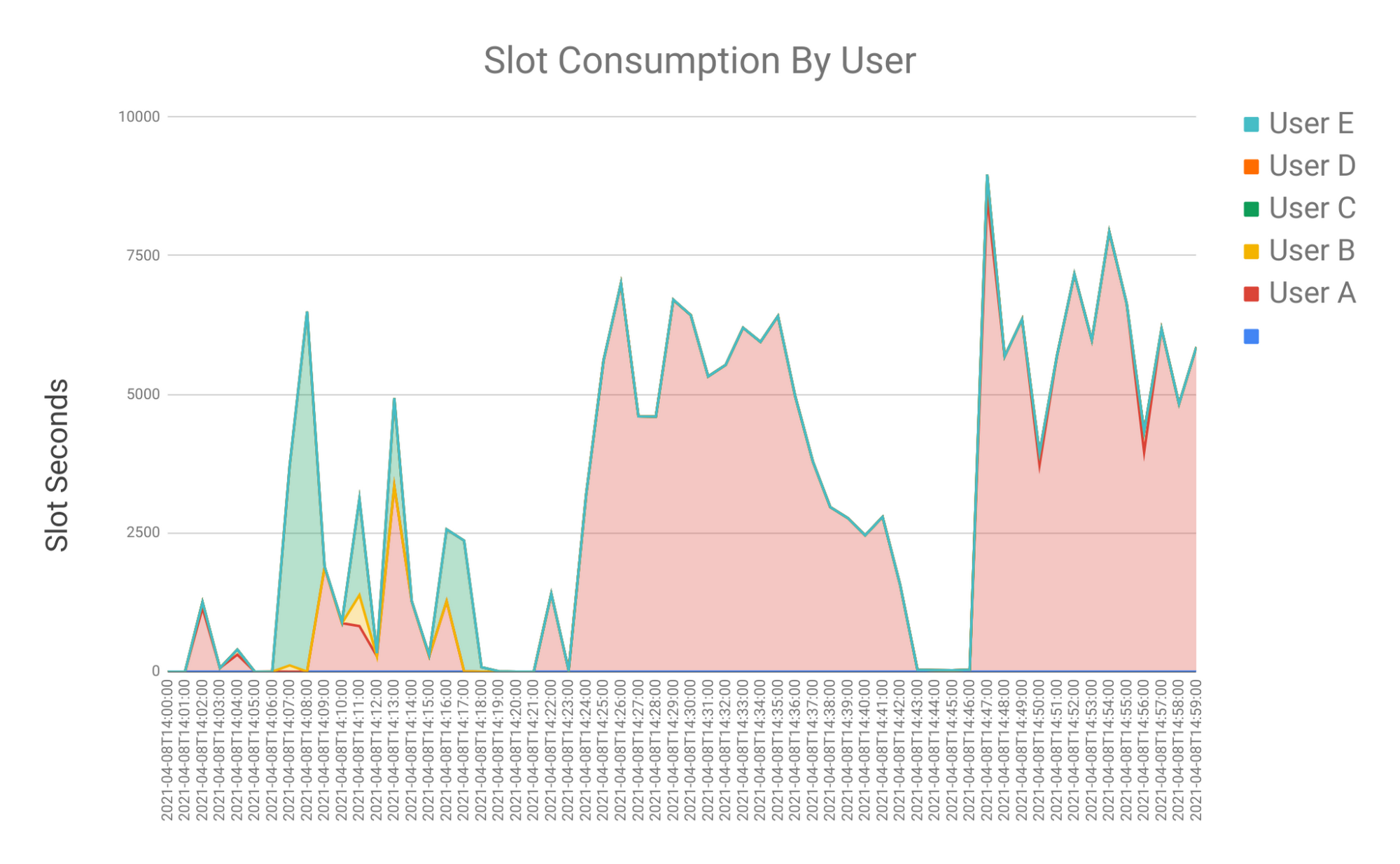
With a little slicing and dicing, you could also produced a Stacked Area Chart By User with Slot Seconds

Analyze / visualize slot consumption and query throughput for an interval of time

The second part of this blog is to monitor the average slot utilization and query throughput for an interval of time. This query will look very similar to the previous query.  The key difference is that we’ll be measuring query count throughput for an interval of time (as opposed to a Point In Time.)  In addition, we’ll measure Total Slot Seconds consumed for that Interval, and we’ll calculate a Pct_Slot_Usage metric (applicable if you are using fixed slots) and an Avg_Interval_Slot_Seconds metric.

Main SQL

Here is the SQL script from the github repo, copy-paste into the BQ UI and run it!

Remember: Change the ‘Region’ qualifier if you aren’t part of the ‘region-US’:

Just like the previous one, let's break down the SQL into smaller chunks for easy understanding. 

Declaring and setting variables

This variable declaration segment is exactly the same as the previous query but with three additions.  We will be using a variable named _RANGE_INTERVAL_MINUTES instead of _RANGE_INTERVAL_SECONDS.  We have added two new variables named ‘_SLOTS_ALLOCATED’ and ‘_SLOTS_SECONDS_ALLOCATED_PER_INTERVAL’.

After declaring, it is time to set these variables.

We’ll discuss the 3 new variables in this section.

• _RANGE_INTERVAL_MINUTES 

As with the last query, the interval size will determine the number of data points on the X-Axis (time); therefore, we want to set the _RANGE_INTERVAL_MINUTES value to something appropriate relative to the Range of time you are interested in analyzing.  If you are only interested in an hour (60 minutes), then a _RANGE_INTERVAL_MINUTES value of 1 is fine, as it will provide you with 60 X-Axis Data Points (one per minute).  However, if you are interested in looking at a 24 hour day (1440 Minutes), then you’ll probably want to set the _RANGE_INTERVAL_MINUTES to something like 10, as it will provide you with 144 X-Axis Data Points.

• _SLOTS_ALLOCATED 

Regarding _SLOTS_ALLOCATED, you will need to determine how many slots are allocated to a specific project or reservation.  For an on-demand project, this value should be set to ‘2000’.  For projects leveraging Flat Rate Slots, you will need to determine how many slots are allocated to the respective project’s reservation.  If your reservation_id only has one project mapped to it, then you will enter a _SLOTS_ALLOCATED value equal to the # of slots allocated to the respective reservation_id.  If multiple projects are linked to a single reservation_id, I’d recommend that you run this query at the ‘ORG’ level (filter on the appropriate reservation_id) and set the variable with the # of slots allocated to the respective reservation_id.

• _SLOTS_SECONDS_ALLOCATED_PER_INTERVAL 

This is simply your interval length converted to seconds multiplied by the number of slots allocated.  This value represents the total number of slot seconds that can be consumed in an interval of time assuming 100% utilization.

Now that all of our variables have been declared and set, we can finally start to analyze the query.   

There are 5 key differences between this query and the “Point In Time” query we reviewed earlier.  

• First, we will not be pulling information at a job_id level.  Given the intended usage of this query, including the job_id granularity would produce query results which would be difficult to dump to a spreadsheet.  

• Second, we will be pulling all timeline values (seconds) within our defined _RANGE_INTERVAL_MINUTES instead of a single second.  This will result in a much more computationally intensive query as we are aggregating much more data.  

• Third, we are counting all queries that ran during our defined_RANGE_INTERVAL_MINUTES instead of just counting the queries actively consuming CPU for a given second in an interval.  This means that the same query may be counted across more than one interval and the ultimate ‘Query_Count’ metric represents the number of queries active during the interval being analyzed.  

• Fourth, we will be calculating a custom metric called ‘Pct_Slot_Usage’ which will sum all slots consumed for an interval and divide that by the number of slots allocated (_SLOTS_ALLOCATED_PER_INTERVAL) for an interval.  For example, for a 10 minute interval given an allocation of 2000 slots, _SLOTS_SECONDS_ALLOCATED_PER_INTERVAL would equate to 1200K Slot Seconds (10 minutes * 60 seconds * 2000 slots.)  During this interval, if we used 600K Slots Seconds, then 600K/1200K equals a ‘Pct_Slot_Usage’ of 50%.  

• Fifth, we will be calculating another custom metric called ‘Avg_Interval_Slot_Seconds’ which will sum all slots consumed for an interval and divide it by _RANGE_INTERVAL_MINUTES * 60 in order to calculate the average slot consumption in Slot Secs for the interval of time.  For example, if a user were to consume 30,000 Slot Seconds in an interval of 5 minutes, the Avg_Interval_Slot_Seconds would equal 100 (30,000 slots consumed / (5 min interval * 60 seconds per minute)).

Note:  It is possible (even likely) that the ‘Pct_Slot_Usage’ metric could have a value greater than 100%.  In the case of an on-demand project, this can occur due to the inherent short query bias built into the scheduler.  

For the first 15-30 seconds of a query’s execution, the scheduler will allow a query to get more than its ‘fair share’ of Slot Seconds (relative to project concurrency and the ‘2000’ slot limit imposed on on-demand projects.)  This behavior goes away for an individual query after 15-30 seconds.  If a workload consists of lots of ‘small’ and computationally intensive queries, you may see prolonged periods of Slot Consumption above the ‘2000’ slot limit.  

In the case of a project tied to a reservation with Fixed Slots, you may see the ‘Pct_Slot_Usage’ metric exceed 100% if Idle Slot Sharing is enabled for the respective reservation and if idle slots are available in the respective Org.

As with the previous script, the outermost query is built from two derived sets of data aliased as ‘key’ and  ‘query_info’.

The ‘key’ derived table

Same as the first query, this derived query is identical to the one used in the previous example.

The query_info derived table

This derived query is very similar to the one in the previous example.  There are 4 key differences.  

• First, we are not selecting JOB_ID.  

• Second, we are looking at all the TimeLine seconds for an interval of time, not a single Point In Time (Second) per Interval as we did in the previous query.  

• Third, in order to get an accurate count of all jobs that ran within an interval of time, we will run a Count Distinct operation on Job_ID.  The ‘Distinct’ piece ensures that we do not count a JOB_ID more than once within an interval of Time.  

• Fourth, in order to match our ‘Period_TS’ value to the key table, we need to aggregate all minutes for an interval and associate that data to the first minute of the interval so that we don’t lose any data when we join to the key table.  This is being done by some creative conversion of timestamps to UNIX seconds, division, and offsets based on which minute an interval starts.

Outermost query  

In the outermost query, we will again LEFT OUTER JOIN the ‘key’ timeline table to our pre-filtered ‘query_info’ table based on the cleaned up TimeStamp values from each table.  This needs to be a LEFT OUTER JOIN versus an INNER JOIN to ensure our timeline is continuous, even if we have no matching data in the ‘query_info’ table.

In terms of the select statement, I’m using our previously defined _UTC_OFFSET value to convert the UTC Timestamps back to our defined TimeZone.  I also select the user_email,  proejct_ID, reservation_ID, Total_Slot_Second, Query_Count, and calculate Pct_Slot_Usage and Avg_Interval_Slot_Seconds.

Similarly like the first query, here are some sample Charts you can create from the final query result:

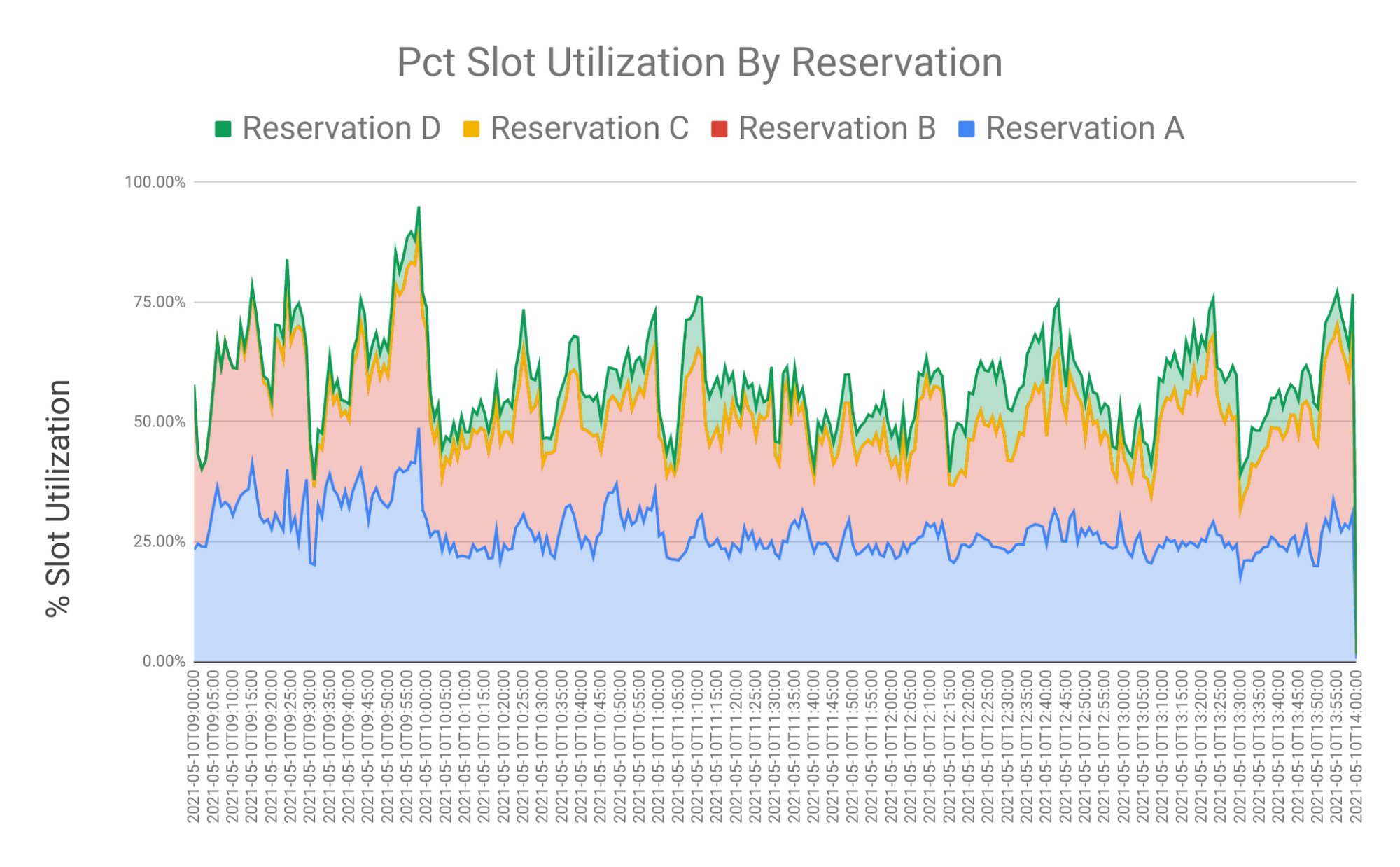
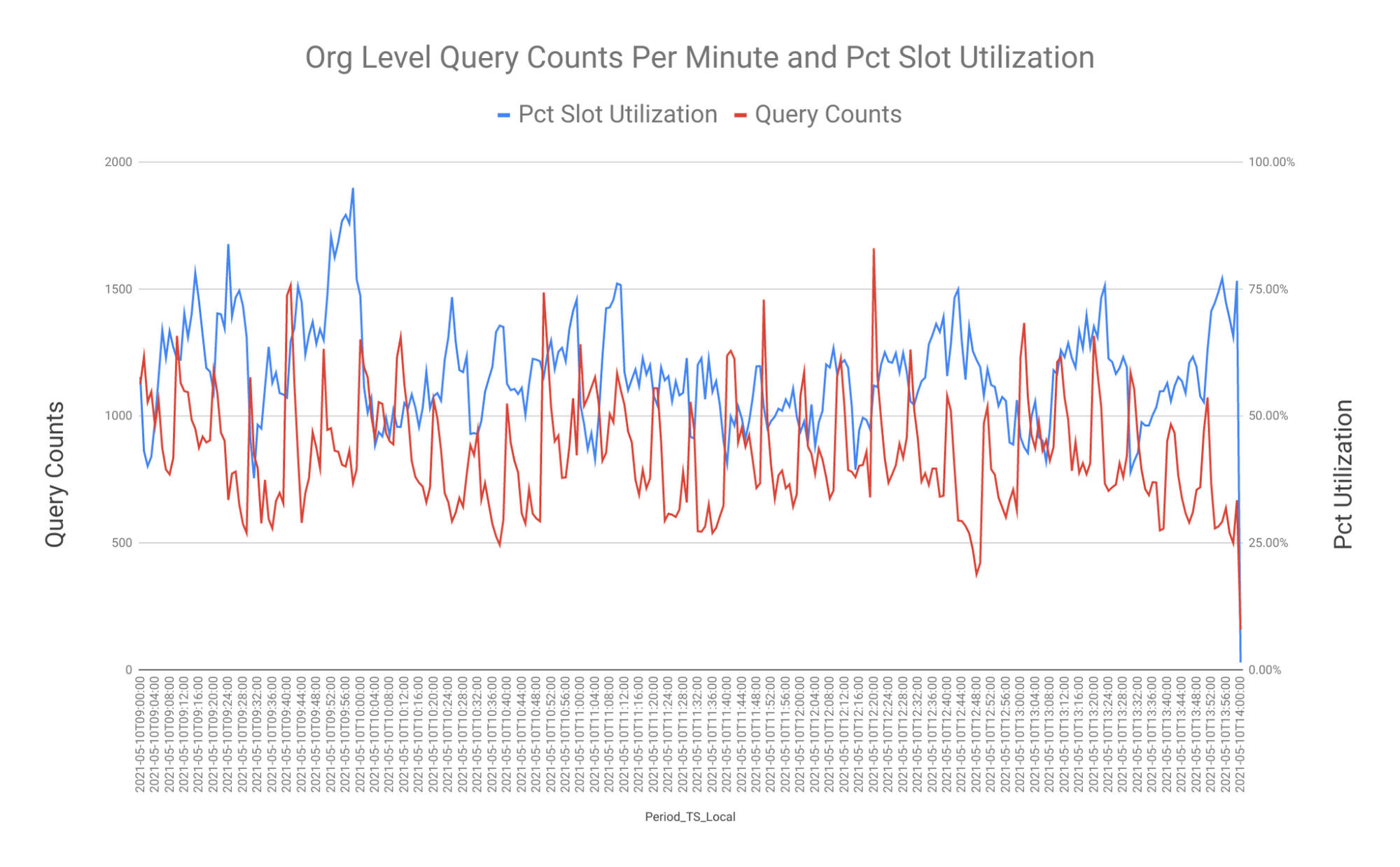
I hope you found these queries and their explanations useful..albeit, maybe a bit wordy.  There was a lot to unpack.  The origin of these queries go back to something similar we use to run on a totally different DBMS.  With BigQuery’s scripting support and Nested Array capabilities, the newly ported queries are much ‘cleaner’. They are easier to read and require many less manual changes to the parameters.  Look out for our future blogs in this series.