Performing prediction with TensorFlow object detection models on Google Cloud Machine Learning Engine

In June, we posted a blog that taught you the basics on training a new object detection model using Google Cloud Machine Learning Engine. Today, we’ll help you take your knowledge one step further. This follow-up blog post will first teach you how to export a trained model into the SavedModel format, then deploy the model on Cloud Machine Learning Engine. Then, you’ll learn how to serve the model and perform prediction by using both online and batch prediction services from Cloud Machine Learning Engine. Let’s get started.

Export the model

Download checkpoint files

This can take a minute or two depending the size of the checkpoint files and your network connection.

Export to the SavedModel model

Three input types are supported in the exporter:

• “image-tensor” — Accepts a batch of image arrays.
• “encoded_image_string_tensor” — Accepts a batch of JPEG- or PNG-encoded images stored in byte strings.
• “tf_example_string_tensor” — Accepts a batch of strings each of which is a serialized tf. Example proto that wraps image bytestrings.

${YOUR_LOCAL_EXPORT_DIR} is the path to which you want to save the exported model, and must not already exist as the exporting program will create the folder for you. Note that the config file specified in --pipeline_config_path must match the one used in training.

Once running successfully, the exporter generates the saved_model.pb under the output_directory/saved_model with possible variable files.

You may want to check to be sure the expected files are in the output folder before proceeding.

You can also inspect the exported model by running saved_model_cli. It will show the input tensor names and output tensor names together with signatures defined. An example command line like the one below will show all available information.

Note that the first dimensions of the input and output tensors should be -1 as this is required by the Cloud Machine Learning engine to support batched-inputs. Also the tensor aliases for input and output tensors are shown in the bracket for each tensor. The aliases (e.g., “inputs”), instead of the actual tensor names (e.g., “encoded_image_string_tensor:0”), are used in the input request or files. This applies to outputs as well.

Prepare the inputs

However, the object_detection model only has one input tensor that accepts one, or a batch, of images. In this case, we can put the image bytes directly in each record without specifying input tensor names. Since this model accepts image bytes for local or online prediction, the input instances should be base64-encoded and packed into JSON objects. An example of the content of the input file would look like:

For batch prediction in this particular case (one string input in the inference graph), the image bytes should be packed into records in TFRecord format and saved into files. The following code shows how to do that in Python. If the inference graph has two or more input tensors, the batch prediction accepts a list of JSON objects just as what local or online prediction does.

For efficiency purposes, this model requires each image in a request have the same heights and widths. Otherwise, the prediction will fail. If you have a lot of images in a variety of sizes, you can resize them with the script shown below. We’ll revisit this requirement later.

The above code generates two files for a given set of images after resizing them to be the same size: one JSON file for local and online prediction, and one TFRecord for batch prediction.

Run local prediction

The inputs should be reasonably small for local prediction, typically containing 2-3 instances. The following shows how to run local prediction using gcloud.

The output shows the prediction results for the two input instances. The detection of the first instances results in 100 objects with the bounding boxes and the corresponding classes and scores. The bounding box values are normalized to [0, 1) and are ordered ymin, xmin, ymax, xmax. The second output row shows the results for the second image sent to prediction.

Run predictions on Cloud Machine Learning Engine

Once you verified the model and a small set of inputs work using "gcloud local prediction", you may proceed to use Cloud Machine Learning Engine to host your model for serving. A model is deployed by creating a Cloud Machine Learning model and version for the exported model. This step is mandatory for online prediction but optional for batch prediction.

First copy the exported model to a Cloud Storage location:

Then, create a model and version in Google Cloud from the exported directory using the following gcloud command. Note that --runtime-version must be specified to be 1.2 as the default TensorFlow version in the service might be older and therefore won't work with this model.

While model creation is instant, it can take 3-5 minutes to create a version. After a version is created, you can run the following to list the models in your project.

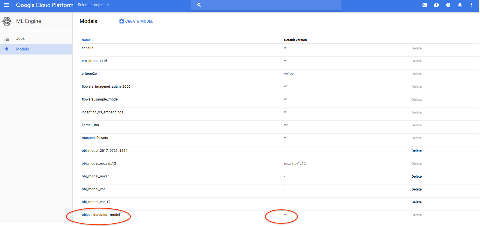
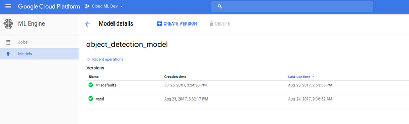
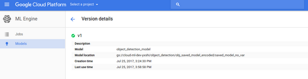
Alternatively, you can go to Cloud Console to see the models and version. Click the model and version to see more detailed information:

Cloud Machine Learning Engine provides a whole set of APIs for model and version management. Please refer to the documentation for more information.

Run online prediction

However, during development, you may find it convenient to use "gcloud" to issue prediction requests to your model, as in the following example command:

The inputs.json is read into the payload of the HTTP request. Model and version information is also embedded there. Upon receiving the request, the service performs inference for all the instances and returns the prediction results to the user in real-time fashion.

Note that the prediction results are re-formatted as a tab-delimited table by the gcloud command line. If you send an http request directly, for example using “curl”, a JSON object is returned which is the same as what you'll find for the prediction result of the batch prediction.

* To craft the payload file for curl command, you need to wrap the instances in JSON into the values of a JSON object with the key being “instances”. See details in this stackoverflow question.

Run batch prediction

Run gcloud command to submit a batch prediction job:

If the job is successfully submitted, you'll see that the job is queued. The command lines to describe the job and stream the logs to your local console are also shown below. Let’s check the job status first:

This shows the job status including the job state, node hours consumed thus far, the number of predicted instances and other information. Example output:

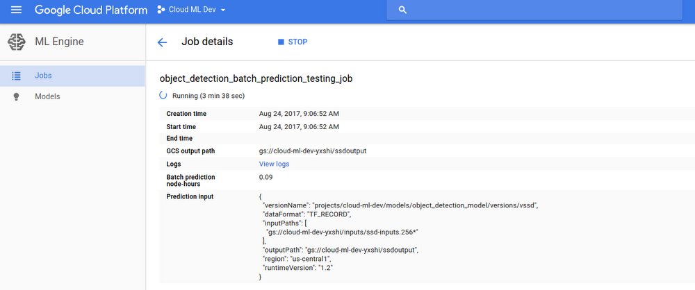
You can also see the job and its status in the Cloud Machine Learning Engine section in Pantheon UI:

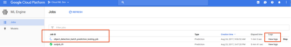
To display the job details, click the Job ID.

Once the job succeeds —  i.e. the output state is SUCCEEDED — check the output Cloud Storage location:

The resultant files contain the prediction results in JSON format. The error stats files contain the error stats, if applicable.

You can also run a batch prediction job without deploying the model. A model dir on Cloud Storage — instead of a model and version — is specified in the request where you’ve saved the model. This is good for faster iteration for batch predictions, but you’ll have to manage the model and version by yourself.

One downside is you may need to explicitly set the runtime version in the request, because the default runtime version might not work for the model. This step is not needed in the case of a deployed model, because the runtime version has been specified when you created the model/version.

Below is the command line to submit a batch prediction job without a model and version:

You should obtain identical prediction results.

Visualize the result

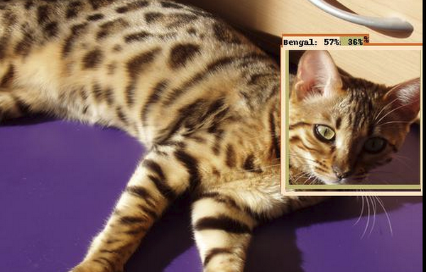
Conclusion

Acknowledgments

This tutorial was created in collaboration with Jonathan Huang from Google Research and Machine Intelligence team and received valuable feedback from Robbie Haertel and Josh Cogan from Google Cloud AI team.