Hyperparameter tuning on Google Cloud Platform is now faster and smarter
Lak Lakshmanan
Director, Analytics & AI Solutions
Wenzhe Li
Software Engineer, Cloud AI
Cloud ML Engine strives to be the best platform for running TensorFlow programs: it provides a serverless environment for machine learning. You can launch a TensorFlow training job or deploy a trained model as a microservice without having to provision a cluster, purchase GPUs, or install any software. In addition to its simplicity of training and deployment, Cloud ML Engine also offers some unique capabilities—hyperparameter tuning being one of them.
Hyperparameter tuning on Google Cloud uses a Bayesian optimization approach that can be applied to autotune parameters (like learning rate, number of hidden nodes, etc.) of your machine learning model. See this blog post for more details on how the Bayesian optimization works.
Recently, hyperparameter tuning has advanced in three ways to become smarter, faster, and more capable. These changes help you obtain more accurate ML models while saving you money. In this blog post, we’ll walk you through these three improvements one at a time, show you how to take advantage of them, and demonstrate the improvements on a machine learning model.
How to use hyperparameter tuning
Before we delve into the improvements, let’s explain how you invoke hyperparameter tuning for your machine learning model. This process consists of four steps:- Ensure that your model writes out evaluation metrics periodically.
- Ensure that the outputs of different trials don’t clobber each other.
- Create a YAML configuration file.
- Submit training job, configuration file included.
1. Write out your evaluation metric
First, make sure that your model outputs evaluation metrics periodically. If you are using a pre-made Estimator in TensorFlow, you can do this by adding code like this:If you are building a custom estimator, you will create an EstimatorSpec which will be be invoked from the train_and_evaluate loop, using code like this:
If you are writing a low-level TensorFlow program (we don’t recommend doing that), you would use tf.summary to export information to checkpoint files. In all these cases, you will be able to visualize in TensorBoard the evaluation metric as your ML model is being trained.
Here, are examples of the evaluation metric for two different models:
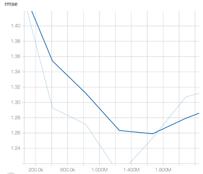
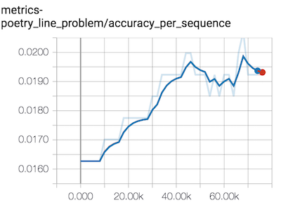
In the first model, the scalar metric is called rmse and in the second model, the scalar metric is called metrics-poetry_line_problem/accuracy_per_sequence. This name serves as the hyperparameterMetricTag that you tell the hyperparameter tuner to optimize. In the case of the RMSE, you’d want to minimize it. In the case of the accuracy per sequence, you’d want to maximize it. So, you’ll have to tell the hyperparameter tuner what your goal is.
2. Don’t clobber outputs
Next, you’ll change your model to get the trial-number from the environment variable and append this trial number to the output directory:This way, the outputs of different trials don’t clobber (overwrite) each other.
3. Create a YAML file
Third, you will identify parts of your model that you want the tuner to change so as to optimize the evaluation metric. For example, you might want the tuner to be able to tune the batch size and the number of embedding nodes in your model. All of these hyperparameters will have to be command-line inputs to your executable Python package. You’d then put these together into a YAML file:Note that the YAML file specifies the name of the metric (rmse) and the goal (to minimize the error). We then give the hyperparameter tuner a budget—to run the training 40 different times, with 5 of them of them in parallel at any time. Finally, we specify the parameters in the model that can be tuned (nembeds, and nnsize) and ranges for each. The tuner will do a Bayesian search in this parameter space to find good combinations of these parameters.
4. Launch your tuning job
Finally, you’ll launch off the hyperparameter tuning job by submitting the job to ML Engine and including the above config file:You can monitor the tuning as it happens. On the web console, you will be able to see the best trial in terms of both the parameters that were used and the objective that was attained. For example, you might see that the best trial was:
This indicates that 40 trials have been completed, and the best so far is trial 35, which achieved an objective of 1.079 with the hyperparameter values of nembeds=18 and nnsize=32.
So, that’s how you use hyperparameter tuning. Now, let’s move on to show you three improvements that have happened in the service and how to take advantage of them.
Faster tuning with early stopping
Typically, when you run a machine learning model, you specify a number of steps (i.e. the total number of batches) that you want the model to be trained over. As the model trains, you evaluate the model and checkpoint it once every, say, 30 minutes. The purpose of checkpointing is twofold: 1) to have an intermediate point to which you can recover in case of machine failure and 2) to provide feedback to the end-user on the training quality. For example, by comparing the loss on the training dataset to the equivalent on the evaluation dataset, it is possible for the end-user to infer overfitting. Machine learning practitioners use the checkpoints both to decide how long to train and how much regularization to carry out.In the context of hyperparameter tuning, there is one additional way to put the checkpoints to use. It is possible to discover that the current trial is unlikely to beat the best model that has already been encountered. Hyperparameter tuning on Cloud ML Engine now cuts short unpromising trials. This means that the next trial can start more quickly, leading to an overall reduction in hyperparameter tuning time. Because your cost depends on how long your job runs, early stopping also makes hyperparameter tuning less expensive. To enable early stopping, simply add a flag to your configuration file:
More cost-effective and efficient tuning by resuming a completed job
One common situation we frequently encounter in hyperparameter tuning is what one of us personally calls bid shading. Bid shading is a common strategy of under-provisioning resources when faced with incomplete information.1 In hyperparameter tuning, you might get full exploration with 100 trials, but it is likely that 50 is enough, so you might do the study with 50 trials to avoid overpaying for 100 trials. Unfortunately, the 50 is only a likelihood and after doing the hyperparameter tuning study with 50 trials, you realize that the best trial was near the end. You are left wondering whether a few more trials would have allowed the autotuner to more completely explore the space. Restarting the hyperparameter tuning, this time with 60 trials, doesn’t appeal because you are essentially paying for the first 50 trials twice.Well, now you can resume a completed study and have it run ten more trials. When you submit the updated job, simply specify the jobId of the previous hyperparameter tuning job and all the exploration that was carried out in the previous job will now be available to your current job:
Resuming a completed job allows the hyperparameter service to start from a much richer starting point, thus providing a shorter, better autotuning run.
Learning from previous trials
Resuming a completed job is an explicit command to the hyperparameter tuner that there is information in a previous study that it should take advantage of. It is helpful when you restart the exact same study, with the exact same parameters. But what if you add a new parameter to the tuning job or want to change the search range?One common situation that we’ve encountered quite often in hyperparameter tuning is that the best value for a parameter ends up being the highest (or lowest) value that we specified. For example, suppose we specified the nembeds variable to be tuned in the range:
Now, if the best trial ends up with nembeds=15, we often want to extend the range and try again.
Simply changing the parameter range to be [3, 30] and re-running the tuning job used to be problematic. The way it used to work was the previously tried values in the [3, 15] range would get tried again. We could avoid this by specifying the range as [15, 30], but that still doesn’t help with the other parameters—the values of batch_size that were attempted earlier will still be attempted. It is difficult to change those ranges because it is possible that the relationship is such that larger values of nembeds requires smaller values of nnsize.
There is still information to be gained from previous runs, but we can no longer simply specify a previously completed trial. Another improvement that has happened in hyperparameter tuning is that the service can now learn from earlier, similar (but not necessarily identical) trials.
To take advantage of this feature, all that you need to do is to name related trials similarly! For example, if you are tuning a model to predict a baby’s birth weight, you might call every training job for this model with a name that starts with “babyweight_regression”. A good convention is to name the jobs like this:
babyweight_regression_$(date -u +%y%m%d_%H%M%S)
Similarly, when tuning a language model to complete lines of poetry
https://cloud.google.com/blog/big-data/2018/02/cloud-poetry-training-and-hyperparameter-tuning-custom-text-models-on-cloud-ml-engine
, you might name every one of the hyperparameter tuning jobs for this model with a name that starts with “poetry_text2text_problem”. Also maintain consistency in parameter names—don’t, for example, change the name from “batch_size” to “batchSize”. As long as you stay consistent when naming your jobs and parameters, and use names long enough that the majority of characters in the job name remain unchanged from one tuning job to the next, hyperparameter tuning will be able to benefit from the exploration carried out in earlier runs.
This feature will also assist your training process if your model has related hyperparameters. For example, in a language model with attention, the number of hidden nodes has to be an exact multiple of the number of attention heads. Suppose we wish to experiment with attention heads in the range [3, 6] and hidden nodes in the range [128, 512]. Providing both these as parameters to the tuner will not work because the tuner might choose 3 attention heads and 128 nodes and 128 is not divisible by 3. Do you see how learning from previous trials can help in this situation?
You could run a hyperparameter tuning job for 3 attention heads and hidden nodes being a discrete set of values such as [150, 300, 450] and then run the next job at 4 attention heads and hidden nodes at [128, 256, 512]. This way, the constraint is satisfied and you get to explore the complete space. Because Bayesian optimization treats the parameters as independent, breaking up a study in this way is a way to impose more complex constraints on inter-parameter relationships.
Measuring the impact of these improvements
So how well do these improvements perform? We hyperparameter-tuned a structured data model the old way with no learning, and the new way, by learning from earlier jobs and early stopping:| Job | Trials | Cost in ML units (USD) | Params for Best RMSE | Best RMSE | Worst RMSE | Comment |
| 1 | 40 | 65.67($32) | nembeds: 3 nnsize: 128 | 1.082 | 2.112 | Isolated job |
| 2 | 40 | 56.55 ($27) | nembeds: 18 nnsize: 32 | 1.079 | 1.823 | Similar to Job 1, except with early stopping enabled. |
| 3 | 20 | 26.83 ($13) | nembeds: 30 nnsize: 32 | 1.079 | 1.631 | Run another 20 trials independent of Job 2. |
| 4 | 20 | 31.05 ($15) | nembeds: 3 nnsize: 32 | 1.077 | 1.231 | Resuming Job 2 to add 20 trials. |
The first row of the table is the “old” way, tuning from scratch without early stopping of trials. As you can see from the second row, on our example, enabling early stopping made hyperparameter tuning cost about 15% less, because the autotuning algorithm is now smarter about choosing which trials to end early.
Once we named our jobs similarly (they all started with the same prefix), the second job learned from the first job. You can see the effect of this learning in the worst RMSE, 1.823, being better than the worst RMSE for the first job (2.112). The second set of 40 trials, in other words, are in a more promising part of the input space than the first even though we didn’t explicitly resume an earlier trial.
The third and fourth rows illustrate the benefit of explicitly resuming trials. In the third row, the set of 20 trials benefits from the previous 40 (note the worst RMSE has continued to get better), but these trials are not an explicit continuation of the previous 40. On the other hand, the job in fourth row is an explicit continuation of Job 2, and so the search space has been considerably pruned. Consequently, the worst RMSE is quite a bit lower. It is also interesting that Job 4 cost a bit more than Job 3. This is because the exploration space is constrained to more promising search areas, and so there were no trials that could be cut short! Your mileage and results will vary, of course, based on on your problem and based on random seeds.
Happy tuning!
1The goal is to reduce problems associated with winner’s curse, where winners tend to overpay in auctions with incomplete information. I play bridge, a card game where auctions with incomplete information happen all the time, so that’s the particular example that occurs to me.


