What’s happening in BigQuery: New federated queries, easier ML, and more metadata

BigQuery, Google Cloud’s petabyte-scale data warehouse, lets you ingest and analyze data quickly and with high availability, so you can find new insights, trends, and predictions to efficiently run your business. Our engineering team is continually making improvements to BigQuery so you can get even more out of it. Recently added BigQuery features include new federated data sources, BigQuery ML transforms, integer partitions, and more.

Read on to learn more about these new capabilities and get quick demos and tutorial links so you can try them yourself.

Query Orc and Parquet files directly with BigQuery

Parquet and ORC are popular columnar open source formats for large-scale data analytics. As you make your move to the cloud, you can use BigQuery to analyze data stored in these formats. Choosing between keeping these files in Cloud Storage vs. loading your data into BigQuery can be a difficult decision. 

To make it easier, we launched federated query support for Apache ORC and Parquet files in Cloud Storage from BigQuery’s Standard SQL interface. Check out a demo:

This new feature joins other federated querying capabilities from within BigQuery, including storage systems such as Cloud Bigtable, Google Sheets, and Cloud SQL, as well as AVRO, CSV, and JSON file formats in Cloud Storage—all part of BigQuery’s commitment to building an open and accessible data warehouse. Read more details on this launch.  

Your turn: Load and query millions of movie recommendations 

Love movies? Here's a way to try query federation: analyze over 20 million movie ratings and compare analytic performance between Cloud SQL, BigQuery federated queries, and BigQuery native storage. Launch the code workbook and follow along with the video. Don’t have a Google Cloud account? Sign up for free.

New data transformations with BigQuery ML

The success of machine learning (ML) models depends heavily on the quality of the dataset used in training. Preprocessing your training data during feature engineering can get complicated when you also have to do those same transformations on your production data at prediction time. 

We announced some new features in BigQuery ML that can help preprocess and transform data with simple SQL functions. In addition, because BigQuery automatically applies these transformations at the time of predictions, the productionization of ML models is greatly simplified.

Binning data values with ML.BUCKETIZE

One decision you will face when building your models is whether to throw away records where there isn’t enough data for a given dimension. For example, if you’re evaluating taxi cab fares in NYC, do you throw away rides to latitude and longitudes that only appear once in the data? One common technique is to bucketize continuous values (like lat/long) into discrete bins. This will help group and not discard infrequent dropoff locations in the long tail:

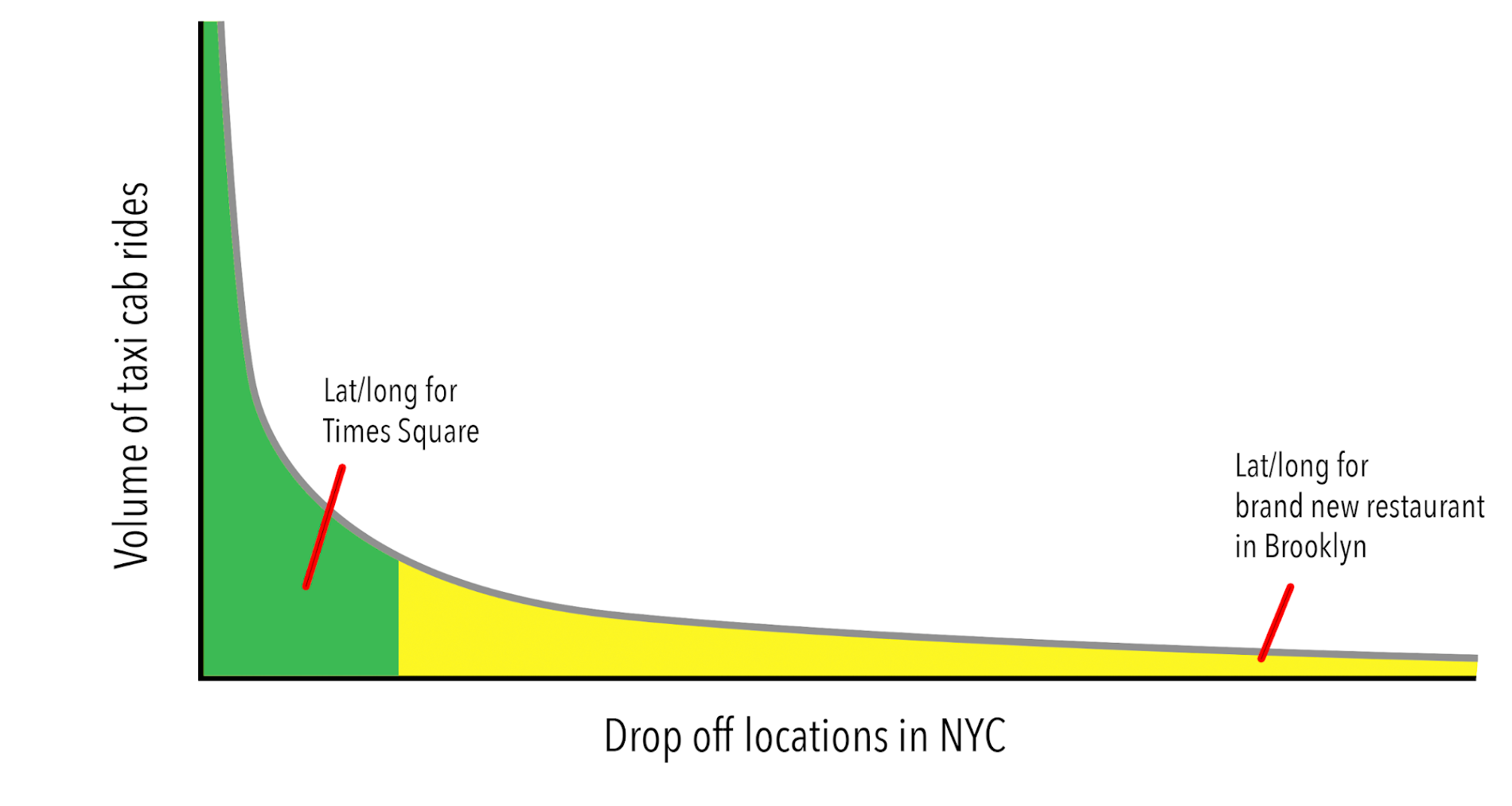
BigQuery provides out-of-the-box support for several common machine learning operations that do not require a separate analysis pass through the data. For example, here’s an example of bucketizing the inputs, knowing the latitude and longitude boundaries of New York:

BigQuery ML now supports running the same preprocessing steps at serving time if you wrap all of your transformations in the new TRANSFORM clause. This saves you from having to remember and implement the same data transformations you did during training on your raw prediction data. Check out the blog post to see the complete example for NYC Taxi cab fare prediction and read more in the BigQuery ML preprocessing documentation. 

Use flat-rate pricing with BigQuery Reservations

BigQuery Reservations is now in beta in U.S. and E.U. regions. BigQuery Reservations allows you to seamlessly purchase BigQuery slots to take advantage of flat-rate pricing and manage BigQuery spending with complete predictability.

BigQuery Reservations allows you to:

• Purchase dedicated BigQuery slots by procuring commitments in a matter of seconds
• Programmatically and dynamically distribute committed BigQuery slots to reservations for workload management purposes
• Use assignments to assign Google Cloud projects, folders, or your entire organization to reservations

Quickly analyze metadata with INFORMATION_SCHEMA

As a data engineer or analyst, you are often handed a dataset or table name with little or no context of what’s inside or how it is structured. Knowing what tables and columns are available across your datasets is a critical part of exploring for insights. Previously, you could select a preview of the data or click each table name in the BigQuery UI to inspect the schema. Now, with INFORMATION_SCHEMA, you can do these same tasks at scale with SQL. 

How can you quickly tell how many tables are in a dataset? What about the total number and names of columns and whether they are partitioned or clustered? BigQuery natively stores all this metadata about your datasets, tables, and columns in a queryable format that you can quickly access with INFORMATION_SCHEMA:

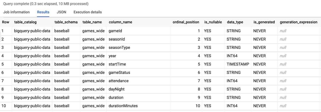
As you can see, with INFORMATION_SCHEMA.COLUMNS there is a list of every column and its data type for all tables in the baseball dataset. 

Let’s expand the previous query to aggregate some useful metrics like:

• Count of tables
• Names of tables 
• Total number of columns
• Count of partitioned columns
• Count of clustered columns

Try the above query with different public datasets like github_repos or new_york or even your own Google Cloud project and dataset. 

Your turn: Analyze BigQuery public dataset and table metadata quickly with INFORMATION_SCHEMA

Practice analyzing dataset metadata with this 10-minute demo video and code workbook. And check out the documentation for INFORMATION_SCHEMA for reference. 

Partition your tables by an integer range

BigQuery natively supports partitioning your tables, which makes managing big datasets easier and faster to query. You can decide which of your timestamp, date, or range of integers of your data to segment your table by. 

Creating an integer range partitioned table

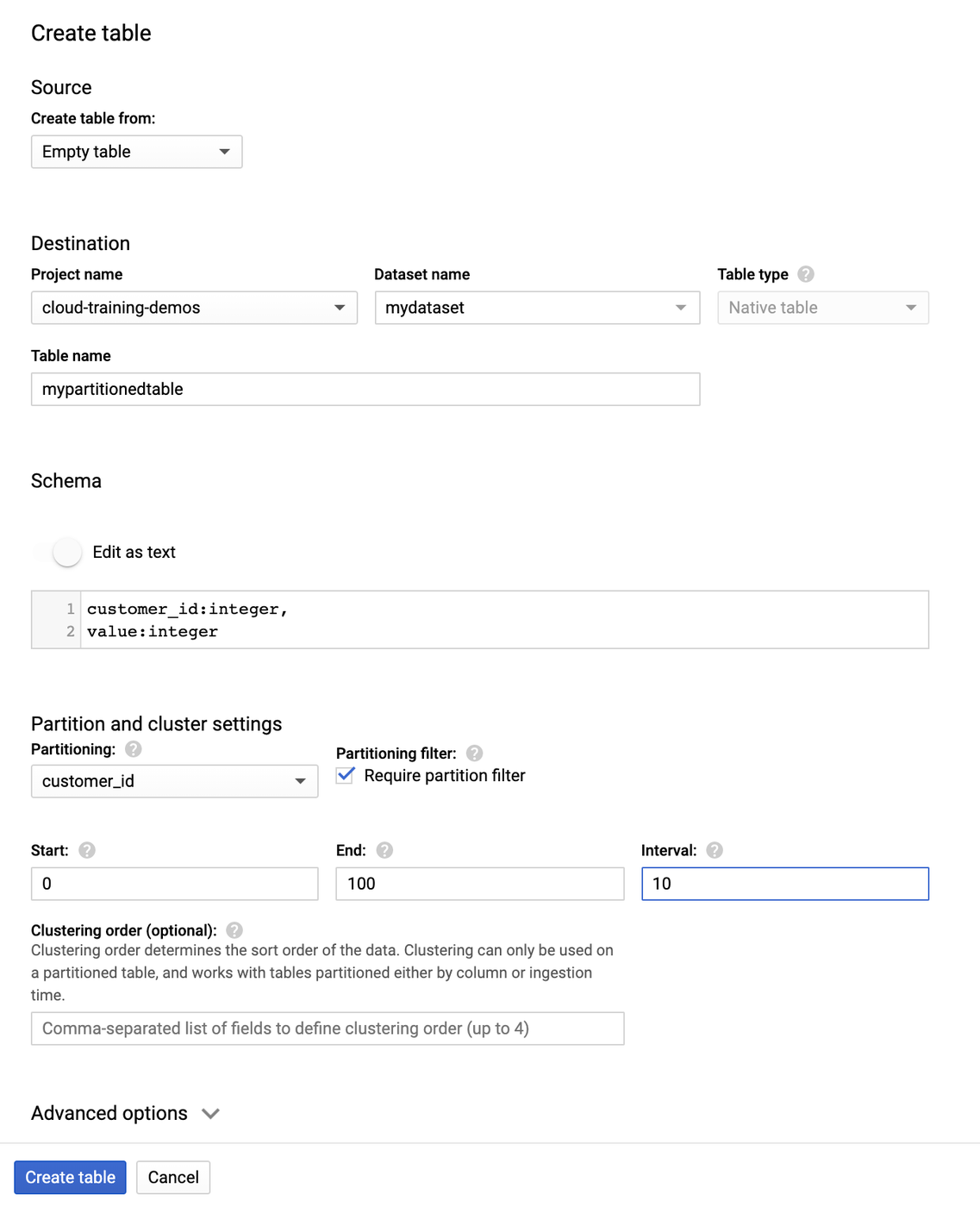
Let’s assume we have a large dataset of transactions and a customer_id field that we want to partition by. After the table is set up, we will be able to filter for a specific customer without having to scan the entire table, which means faster queries and more control over costs.

Here we create an integer range partitioned table named mypartitionedtable in mydataset in your default project. Here’s how you create the table using the Console UI:

And here is the equivalent command using the BigQuery CLI:

The partitioning is based on a start of 0, end of 100, and interval of 10. That means we have customer IDs from 0 to 100 and want to segment them in groups of 10 (so IDs 0-9 will be in one partition, and so on.). Note that new data written to an integer range partitioned table will automatically be partitioned. This includes writing to the table via load jobs, queries, and streaming. As your dataset changes over time, BigQuery will automatically re-partition your data too.

Using table decorators to work with specific partitions 

You can use table decorators to quickly access specific segments of your data. For example, if you wanted all the customers in the first partition (0-9 ID range) add the $0 suffix to the table name:

This is particularly useful when you need to load in additional data—you can just specify the partitions using decorators. 

For additional information about integer range partitions, see Integer range partitioned tables.