Distributed optimization with Cloud Dataflow
Joachim van der Herten
Chief Technology Officer, ml2grow.com
Optimization problems aim to find values for parameters of a system, such that a given aspect (the objective) of the problem is maximized (or minimized). When some of the parameters of the system are restricted to a discrete set of values rather than a range, applying algorithms such as gradient descent directly can be problematic. This type of optimization problem is typically called a mixed integer programs, and the most straightforward method to find a solution is to perform a search over the grid formed by the discrete values:
- Form a grid with all possible values for the discrete parameters.
- Optimize the non-discrete parameters for each item of the grid with—for instance—gradient descent.
Naturally, the grid grows considerably in size if the number of discrete parameters increases: as a consequence, the computational demands grow significantly when a large number of continuous optimization problems need to be solved. Fortunately, this pattern allows distributing the workload over several nodes. As shown below, Cloud Dataflow offers a very flexible and serverless way to accomplish this: the Python SDK consists of transforms that allow simple integration with the rich ecosystem of data and scientific processing Python libraries including NumPy, SciPy, Pandas, or even TensorFlow.
Case study
Consider a set of crops that will need to be harvested at the end of the season, and which must be distributed optimally over a set of available greenhouses. Once the crops have been assigned to a greenhouse, some production parameters can be tuned for each greenhouse to increase the efficiency (minimize cost and maximize yield). The goal is to map all the crops across the greenhouses to obtain maximal efficiency, given transportation costs and other constraints.
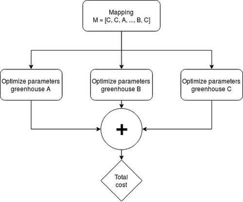
It’s possible to represent the assignment of crops to greenhouses as discrete parameters: each crop is in one greenhouse. A single configuration of all crops assigned to a greenhouse is referred to as mapping and represented as a list. Each element corresponds to a single crop assigned to a greenhouse:
M=[C,C,A,...,B,C]
The efficiency of a greenhouse can be simulated as a function of continuous parameters, and can be optimized with gradient descent.


For a problem with N crops and M greenhouses, MN mappings can be formed. For each mapping, the production parameters for M greenhouses need to be solved, meaning the upper bound for the number of gradient descent problems equals M(N+1), assuming production of each crop be possible in every greenhouse.
Setting up the pipeline
The Apache Beam pipeline is structured as follows:
Generate all possible mappings of crops to greenhouses
For the greenhouses in each mapping, optimize the production parameters
Include transportation costs
Aggregate by mapping and sum the costs
Aggregate all mappings and select the mapping with minimal cost
The starting point for your pipeline is a comma separated (CSV) file, with each line representing a crop. The first column is the crop name, the second the total amount to be produced expressed in tons, followed by columns representing the transportation cost per unit if the crop were to be produced in that greenhouse. An empty column indicates the crop can not be produced in the specified greenhouse.


This information is used to produce all possible lists describing the mappings, which are further transformed into a PCollection of the following data structure, representing a single optimization task to be solved with gradient descent:
((<mapping ID>, <greenhouse>), [(crop, quantity),...])
ParDo, these tasks are solved with a standard solver from SciPy:Thus, the Python SDK for Dataflow provides a simple interface to integrate the solver, with no additional requirements in terms of implementation. This example uses SciPy, but it is even possible to construct a TensorFlow graph and run computations with it inside a ParDo. Other transforms of the SDK such as Map, side-inputs, and GroupBy provide a flexible way to process and organize the input for the solver.
Additionally, these transforms are similar to functional programming constructs in Python, which might help you find them familiar. As a very large number of these tasks need to be executed, it makes sense to distribute the workload. Cloud Dataflow automatically takes care of this in a serverless manner, which means there’s not need to manage infrastructure and install distributed frameworks. Additionally, the amount of hardware available becomes less a limiting factor: even for large grids, Dataflow will automatically scale up to the suitable number of computing nodes to parallelize execution.
Summary
The Beam paradigm offers a very flexible way to parallelize and scale optimization workloads that can be split up into many tasks in a serverless manner with no need to manage infrastructure. Mixed integer programming is a prime example of this class of problems. Even our limited example requires us to evaluate a large solution space. Cloud Dataflow’s Python SDK provides transforms familiar to most Python developers, and permits easy integration with the rich ecosystem of data-processing and scientific-processing libraries.
The exhaustive search over the discrete solution grid we discussed in this example has its limits: the size may quickly grow beyond what is feasible, even with the scalability offered by Dataflow. Note, however, that the same approach described in this blog post can be used to efficiently scale the computation of fitness values for an entire generation in the context of population-based algorithms such as genetic algorithms and evolutionary strategies. These algorithms can be used as more efficient alternatives to search through the discrete grid.


