Hyperparameter tuning in Cloud Machine Learning Engine using Bayesian Optimization
Puneith Kaul
Software Engineering Manager
Daniel Golovin
Staff Software Engineer, Google Brain
Cloud Machine Learning Engine is a managed service that enables you to easily build machine learning models that work on any type of data, of any size. And one of its most powerful capabilities is HyperTune, which is hyperparameter tuning as a service using Google Vizier. Hyperparameter tuning is a well known concept in machine learning and one of the cornerstones of architecting a machine learning model. A good choice of hyperparameters can really make an algorithm shine. One of the advantages of Cloud ML Engine is that it provides out-of-the-box support for hyperparameter tuning using a simple YAML configuration without any changes required in the training code.
The beauty of using Cloud ML Engine is that you don’t necessarily need an advanced math background to get the most from hyperparameter tuning. But if you do have a math background, or are just curious about how it all works, this blog post provides an overview of Bayesian optimization, what’s under the hood in Cloud ML Engine and why it’s a state-of-the-art approach.
Hyperparameter overview
But first, let’s quickly recap what hyperparameters are. Hyperparameters are parameters of the training algorithm itself that are not learned directly from the training process. Imagine a simple feed-forward neural network trained using gradient descent. One of the hyperparameters in the gradient descent is the learning rate, which describes how quickly the network abandons old beliefs for new ones. The learning rate must be set up-front before any learning can begin. So finding the right learning rate involves choosing a value, training a model, evaluating it and trying again.
Why hyperparameters are important
Hyperparameter selection is crucial for the success of your neural network architecture, since they heavily influence the behavior of the learned model. For instance, if the learning rate is set too low, the model will miss important patterns in the data, but if it's too large, the model will find patterns in accidental coincidences too easily. Finding good hyperparameters involves solving two problems:
- How to efficiently search the space of possible hyperparameters (in practice there are at least several hyperparameters, and they interact with each other).
- How to manage a large set of experiments for hyperparameter tuning.
Cloud ML Engine addresses both problems using a single command as shown here.
Simpler approaches
At Google, we use Bayesian optimization for implementing hyperparameter tuning. But before we get into what that is and why we use it, let’s talk first about other naive methods of hyperparameter tuning.
One very traditional technique for implementing hyperparameters is called grid search. Grid search is essentially an exhaustive search through a manually specified set of hyperparameters. Let's assume you have a model with two hyperparameters learning_rate and num_layers. Grid search requires us to create a set of two hyperparameters
Grid search then trains the algorithm on each pair (learning_rate, num_layers) and measures performance either using cross-validation on training set or a separate validation set. The hyperparameter setting which gives the maximum score is the final output. This is a very simple algorithm and suffers from the curse of dimensionality, though it's embarrassingly parallel
Grid search exhaustively searches through the hyperparameters and is not feasible in high dimensional space. By contrast, random search, which simply samples the search space randomly, does not have this problem, and is widely used in practice. The downside of random search, however, is that it doesn’t use information from prior experiments to select the next setting. This is particularly undesirable when the cost of running experiments is high and you want to make an educated decision on what experiment to run next. It’s this problem which Bayesian optimization will help solve.
Bayesian optimization in Cloud Machine Learning Engine
At Google, in order to implement hyperparameter tuning we use an algorithm called Gaussian process bandits, which is a form of Bayesian optimization.Wait, what? So what are we trying to solve?
We want to select hyperparameters that give the best performance. This amounts to an optimization problem, specifically, the problem of optimizing a function f(x)(i.e., performance as a function of hyperparameter values) over a compact set A, which we can write mathematically as
Many optimization settings, like the one above, assume that the objective function f(x) has a known mathematical form, is convex or is cheap to evaluate. But the above characteristics do not apply to the problem of finding hyperparameters where the function is unknown and expensive to evaluate. This is where Bayesian optimization comes into play.
Bayesian optimization is an extremely powerful technique when the mathematical form of the function is unknown or expensive to compute. The main idea behind it is to compute a posterior distribution over the objective function based on the data (using the famous Bayes theorem), and then select good points to try with respect to this distribution.
Gaussian processes
To use Bayesian optimization, we need a way to flexibly model distributions over objective functions. This is a bit trickier than modeling a distribution over, say, real numbers, since we’ll need one such distribution to represent our beliefs about f(x) for each x. If x contains continuous hyperparameters, there will be infinitely many x for which we must model f(x), i.e., construct a distribution for it. For this problem, Gaussian processes are a particularly elegant technique. In effect, they generalize multidimensional Gaussian distributions, and versions exist that are flexible enough to model any objective function. Originally GPs were developed to help search for gold; we use them to look for machine learning gold.
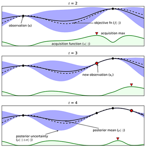
In the above figure, let’s imagine we have an unknown objective function denoted by the dotted line, which is the actual reward the agent will receive. Our goal objective is to find that maximum reward.
Exploration-exploitation tradeoff
Once we have a model for the objective function, we need to select a good point to try. This creates an exploration-exploitation tradeoff similar to one you face when selecting a restaurant: Do you eat at your usual place (which is reliably good), or take a risk and try the new one (which might be great, or might be terrible)?
We know from the Gaussian process the predicted distribution for the observed value at xt+1 given the first t observations, Dt is

The expression for ? and ? is below, where K and k are a kernel matrix and vector derived from a positive definite kernel, ? . In particular K is a t by t matrix with Kij = ?(xi, xj) and k is a t-dimensional vector with Ki = ?(xi, xt+1). Finally, y is the t-dimensional vector of observed values.
The above probabilistic distribution says that after conditioning on the data you have, the predicted value y for a test point x is distributed as a Gaussian. And this Gaussian has two statistics mean and variance. Now, in order to trade off exploration-exploitation we need to choose the next point balancing where mean is high (exploitation) and where the variance is high (exploration).
Acquisition function
To encode the tradeoff between exploration and exploitation, we can define an acquisition function that provides a single measure of how useful it would be to try any given point. We can then repeatedly find the point that maximizes this acquisition function and try it next. Here are a few possibilities:
Upper confidence bound
Perhaps the simplest acquisition function looks at an optimistic value for the point. Given a parameter beta, it assumes the value of the point will be beta standard deviations above the mean. Mathematically, it is
By varying beta, we can encourage the algorithm to explore or exploit more.
Probability of improvement
The main idea behind probability of improvement acquisition function is that we pick the next point based on the maximum probability of improvement (MPI) with respect to the current maximum.
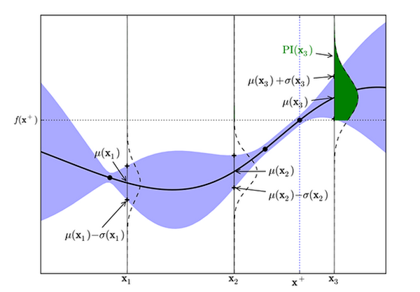
Figure 2: Probability of improvement for a Gaussian Process (from Eric Brochu, Cora and Freitas 2010)
In the above figure, the maximum observed value, y+ is at x+. The area of the green shaded region gives the probability of improvement at x3. The model predicts negligible possibility of improvement at x1 or x2. Whereas sampling at x3 is likely to produce an improvement over y+.
Where ?(.) is normal cumulative distribution function.
Expected Improvement
The algorithm which Cloud ML Engine uses for acquisition function is an implementation in Google Vizier called Expected Improvement. It measures the expected increase in the maximum objective value seen over all experiments, given the next point we pick. In contrast, MPI only takes into account the probability of improvement and not the magnitude of improvement for the next point. Mathematically, as proposed by Mockus, it is

where the expectation is taken over Yt+1 which is distributed as the posterior objective value at xt+1 In other words, if the objective function were drawn from our posterior distribution, then EI (x) measures the expected increase in the best objective we have found during entire tuning run if we select x and then stop.
When using a Gaussian process we can obtain the following analytical expression for EI
Where Z(.) has the expression denoted below and ?(.) and ?(.) denote the PDF and CDF of the standard normal distribution function.
Conclusion
Hopefully this blogpost gave you a little insight into how Cloud ML Engine implements state-of-the-art algorithms for hyperparameter tuning so you can develop powerful machine learning models with far less effort. Moreover, Cloud ML hyperparameter tuning will continue to improve as we at Google conduct ongoing fundamental research in this area and incorporate it into HyperTune.
If you’re interested in learning more, check out the references and resources below.
References
- Google Vizier: A Service for Black-Box Optimization
- Parallelizing Exploration–Exploitation Tradeoffs with Gaussian Process Bandit Optimization
- A Tutorial on Bayesian Optimization of Expensive Cost Functions, with Application to Active User Modeling and Hierarchical Reinforcement Learning
- Youtube: Machine Learning - Bayesian optimization and multi-armed bandits