Deep reinforcement learning on GCP: using hyperparameter tuning and Cloud ML Engine to best OpenAI Gym games

Like many other areas of machine learning research, reinforcement learning (RL) is evolving at breakneck speed. Just as they have done in other research areas, researchers are leveraging deep learning to achieve state-of-the-art results. In particular, reinforcement learning has significantly outperformed prior ML techniques in game playing, reaching human-level and even world-best performance on Atari, beating the human Go champion, and is showing promising results in more difficult games like Starcraft II. Furthermore it’s also helped advance fields like self driving cars, recommendation systems, bidding, and even Machine Learning model development.

Training deep RL agents can be expensive in terms of both computing resources and time. It is common for an algorithm to take tens of thousands or millions of simulation/training steps before one observes the accumulated rewards start to rise. And it can take a lot more from there for the algorithm to converge. For example, in a paper from DeepMind they indicated it took approximately 20 epochs (1 epoch = 0.5 hour according to the paper) before the agent showed clear signs of learning. The entire process took 100 epochs, and yet that was only a single trial!

Furthermore, RL problems are notoriously sensitive to hyperparameters, which means it’s necessary to evaluate many different hyperparameters.

Using these factors as motivation, in this post, we show how to train many jobs in parallel using Google Cloud’s hyperparameter tuning service with ML Engine. This service gives you two key benefits:

• You can train many models in parallel, this allows you to quickly iterate your concept and you only pay for the compute resources you use in each job.
  
• You benefit from the managed hyper-parameter tuning service, which typically results in quicker convergence than just using a naïve grid search.
  

While these properties are beneficial for all machine learning problems, they are particularly beneficial for reinforcement learning problems where the compute is intensive and it’s often necessary to run many trials, evaluating different hyperparameters.

All of the code for this post is located in the GitHub repository here and here. The code provides examples for using RL on GCP; it could be refined for better results.

Reinforcement learning 101

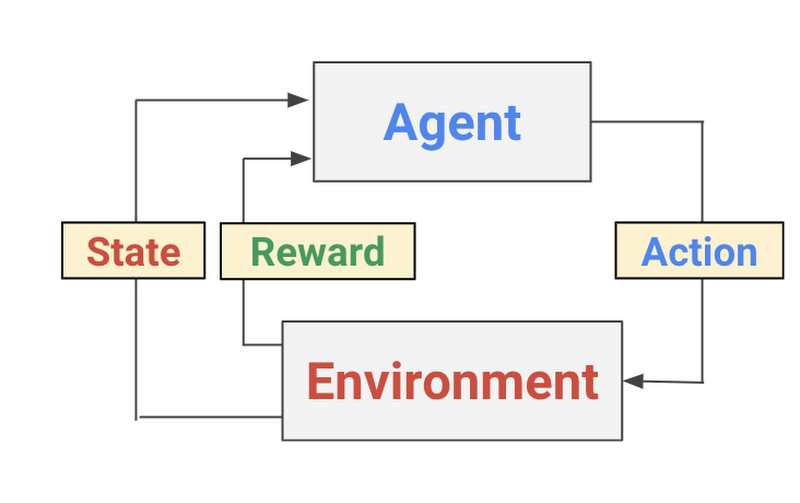
Reinforcement learning (RL) is a form of machine learning whereby an agent takes actions in an environment to maximize a given objective (a reward) over this sequence of steps. Unlike more traditional supervised learning techniques, every data point is not labelled and the agent only has access to “sparse” rewards. While the history of RL can be dated back to the 1950s and there are a lot of RL algorithms out there, 2 easy to implement yet powerful deep RL algorithms have a lot of attractions recently: deep Q-network (DQN) and deep deterministic policy gradient (DDPG). We briefly introduce the algorithms and variants based on them in this section.

What is a Deep Q-network?

The Deep Q-network (DQN) was introduced by Google Deepmind’s group in this Nature paper in 2015. Encouraged by the success of deep learning in the field of image recognition, the authors  incorporated deep neural networks into Q-Learning and tested their algorithm in the Atari Game Engine Simulator, in which the dimension of the observation space is very large. The deep neural network acts as a function approximator that predicts the output Q-values, or the desirability of taking an action, given a certain input state. Accordingly, DQN is a value-based method: in the training algorithm DQN updates Q-values according to Bellman’s equation, and to avoid the difficulty of fitting a moving target, it employs a second deep neural network that serves as an estimation of target values. This network’s weights are updated only at a specified interval and hence helps training the DQN. Since RL collects data by interacting with the environment continuously, its data is time-correlated, which can prevent the DQN from converging during training. To address this problem, the authors introduced a replay buffer to hold data previously collected and then sample mini-batches from it during each training iteration. For more details on the techniques the DeepMind group used to build this successful strategy, take a look at this paper.

DDPG, TD3 and C2A2

Like DQN, DDPG is a value-based RL method. To be concrete, it is an actor-critic method where the actor is responsible for making decisions on actions given a state from the environment and the critic estimates the value of a given state (or a pair of state and action). Similar to DQN, DDPG uses deep neural networks as its function approximators for both the actor and the critic.

One major problem of DDPG is that the critic tends to overestimate in the learning process (this is actually a problem observed in most value-based RL methods, including DQN). To address this, Twin Delayed Deep Deterministic policy gradient (TD3) proposes to have 2 critics and whenever a (state, action) pair is given the minimum of which is regarded as the estimated value (line 06-11). Besides this, TD3 also proposes to delay the update of its target networks to reduce the growth of estimation error as well as target policy smoothing regularization to prevent overfitting to narrow peaks in the value estimation. You can learn more about TD3 in this paper.

TD3 works great and is easy to implement. But it would be better (and fun!) to have options over actions when the agent thinks the estimated value is low. We therefore added one more actor to TD3 and dub the algorithm as C2A2 (for an apparent reason). C2A2 has the same way of value estimation as TD3, but the extra actor provides it with choices over actions where the agent picks the one with larger estimated value. This logic is revealed in line 18-27, it demonstrates the fact that creating a new algorithm to run on Cloud ML engine requires no specific code modification to suit for the platform.

Deep RL in the OpenAI gym environment

OpenAI gym is a popular platform for people to try/evaluate RL algorithms. Using OpenAI Gym, we can initialize an environment for our agent to interact with:

Assuming we have already trained our agent, it will select an action using the observations from the environment as inputs:

Steps to run RL on Cloud ML Engine

Running a hyperparameter tuning job on Google Cloud is straightforward. Here are the 5 steps you’ll need to take:

1. Build your model in a normal way.

2. Establish your hyperparameters as command line arguments, thereby decoupling your hyperparameters from your model’s logic

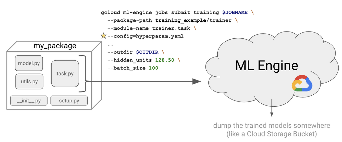
3. Create a Python package (i.e., add a __init__.py and setup.py)

4. Write your hyperparameter.yaml file

5. Submit your first training job from the command line using gcloud ml engine submit

In practice, you will typically spend most of your time on step 1, whereas  you can start with boilerplate code for the rest of the process. In our setup, we have implemented simple policy gradients agent and a DQN agent compatible with OpenAI’s gym library, as well as TD3 for continuous control problems. You can check out the implementations here and here.

Hyper-Parameter Tuning: Preparing your code

Once you’ve written your reinforcement learning agent and defined the task that you want to solve, you then need to set up your hyperparameters as command-line arguments. This will be crucial because it allows us to decouple all the hyperparameters from one another, thus allowing us to evaluate the effect of each hyperparameter independently. For example using the argparse library, hyperparameters can set as command line arguments:

For hyperparameter tuning, there are two important additions we need to add to the model: 1) specify the metric we want to optimize on; and 2) give each model output a unique name.

You may want to add a custom metric: in our case, we’ll call it the reward. This can be accomplished like so:

Alternatively, if you are using TensorFlow, you simply need to log your metric as you would for TensorBoard:

Below, we will tell ML Engine to optimize over this reward parameter in a YAML file.

Additionally we need to package up our code into a Python package. You can read more about this process here, but essentially it means we need to add an empty __init__.py file and a setup.py to our folder structure. So here are the latest modifications  to our code:

Hyper-Parameter Tuning: Submitting a Job

Now that we have created our model, we will define a hyperparameter yaml file that indicates which hyperparameters we want to tune, the value ranges for each hyperparameter, and which metric we want optimize (“reward” in RL’s case).

Additionally, here you can also specify the scale-tier, which indicates how much compute power you want to use. In our case, we are going to use a single GPU for each job. If you wanted a custom setup, with multiple GPUs, for example, you can specify a custom scale tier. A nice benefit of using ML Engine for machine learning is that it allows you to focus on model development and deployment without worrying about infrastructure.

It’s important to note that the hyperparameter tuning service, because it’s using Bayesian optimization, is a sequential algorithm that learns from each prior step. Thus you must specify the maxTrials and the maxParallelTrials.

In the extreme case, if the maxParallelTrials is equal to maxTrials the process will finish quickly, in about the time it takes to train a single model (in this case you can set the algorithm parameter to GRID_SEARCH to perform grid search instead of Bayesian optimization).  Conversely, if your maxParallelTrials parameter is small, it will take longer to train, but will generally result in better performance as its Bayesian optimization process has benefited from more epochs from which it was able to incrementally improve the model. Here is an example:

The YAML file specifies the name of the metric (“reward” in the case of RL) and the goal (to maximize this metric). We are also giving the hyperparameter tuner a budget—we are allowing it to train 40 total models, with 5 of them run in parallel at any time. Finally, we specify the hyperparameters in the model that can be tuned (learning_rate, batch_size, etc.), along with ranges for each hyper-parameter.

Lastly, we are now ready to submit a hyperparameter job on ML engine:

Notice we have the --config argument where we point to our hyperparameter yaml file. Essentially the process will fire off various training jobs using different hyperparameters.

You can view the job status into primary ways:

• From the command line
  
• From Cloud Console

Can our model play successfully?

We wrote three reference examples for running reinforcement learning on GCP:

1. A very simple policy gradients implementation to solve Cartpole using OpenAI Gym in TensorFlow
   
2. A more advanced DQN implementation to solve BreakoutGym environments using tf.keras
   
3. TD3 using TensorFlow in the BipedalWalker environment
   

We will share our results from all three implementations including the hyperparameter tuning results, along with visualization of agents solving Cartpole, Breakout, and BipedalWalker.

Because we wrote all of our jobs to model directories on Cloud Storage, we can visualize the trial results using TensorBoard:

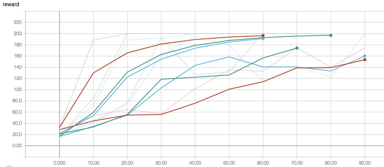
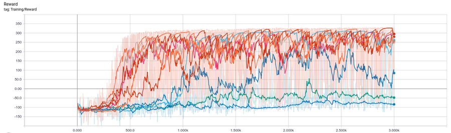
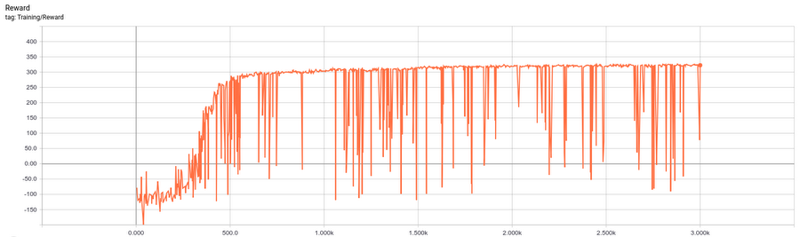
Learning curve from the best of the above trials. BipedalWalker is considered “solved” if the agent can continuously reach an average reward of 300 for 100 episodes in a row. The agent we trained meet the criteria before episode #2000 and this can put us at the third place (at the time of writing 2018-12-10) on the leaderboard. Try modifying the hyper-parameter tuning configurations here and see if you can earn a higher score.

It can be a bit hard to interpret evaluation curves for multiple trials, so often we simply look at the final objective value. We can view our final results in ML Engine > Jobs on the Cloud Console:

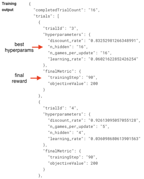
Example outputs as viewed on Cloud Console.

Reinforcement learning posts aren’t nearly as fun when they omit some GIF animations of our agent playing a video game, so we’ll introduce some now. For our policy gradients implementation with CartPole, the best parameters—limited to using only 30 gradient steps (given enough iterations, CartPole will reach the terminal 200 reward even with suboptimal hyperparameters)—were:

In contrast, using suboptimal hyperparameters the environment finished before reaching the terminal state, reaching a reward of only 32:

Additionally, we also built a DQN implementation to solve more complex Gym environments. We ran our code on Breakout, and below are a couple of our results using the better hyperparameters. Performance could no doubtly improve with longer training and searching a larger hyperparameter space.

Results from BipedalWalker:

After only 100 episodes of training, the agent could barely stand.

After training for 1000 episodes, the agent is able to finish the course (in an inefficient way).

The agent’s gait became agile after training for 2000 episodes.

Conclusion

Reinforcement learning is currently undergoing a really exciting period of rapid innovation. ML Engine serves as a valuable tool for practitioners and researchers working on solving problems with reinforcement learning. Specifically, the hyperparameter tuning service in ML Engine allows users to evaluate different types of hyperparameter combinations, while also benefiting from the managed hyper-parameter tuning service using Bayesian optimization that speeds up optimization process compared to a naive grid search. For more information on hyperparameter tuning, check out this documentation page.

Additional Resources

• Machine Learning with TensorFlow on GCP
  
• Hyperparameter tuning on GCP
  
• How to train ML models using GCP